Chapter 6 Simulation
Simulation is a computer-based, computationally intensive, method of solving difficult problems, such as analyzing business processes. Instead of creating physical processes and experimenting with them in order to understand their operational characteristics, a simulation study is based on a computer representation - it considers various hypothetical conditions as inputs and summarizes the results. Through simulation, a vast number of hypothetical conditions can be quickly and inexpensively examined. Performing the same analysis with a physical system is not only expensive and time-consuming but, in many cases, impossible. A drawback of simulation is that computer models are not perfect representations of business processes.
There are three basic steps for producing a simulation study:
Generating approximately independent realizations that are uniformly distributed
Transforming the uniformly distributed realizations to observations from a probability distribution of interest
With the generated observations as inputs, designing a structure to produce interesting and reliable results.
Designing the structure can be a difficult step, where the degree of difficulty depends on the problem being studied. There are many resources, including this tutorial, to help the actuary with the first two steps.
6.1 Generating Independent Uniform Observations
We begin with a historically prominent method.
Linear Congruential Generator. To generate a sequence of random numbers, start with \(B_0\), a starting value that is known as a “seed.” Update it using the recursive relationship \[B_{n+1} = a B_n + c \text{ modulo }m, ~~ n=0, 1, 2, \ldots .\] This algorithm is called a linear congruential generator. The case of \(c=0\) is called a multiplicative congruential generator; it is particularly useful for really fast computations.
For illustrative values of \(a\) and \(m\), Microsoft’s Visual Basic uses \(m=2^{24}\), \(a=1,140,671,485\), and \(c = 12,820,163\) (see http://support.microsoft.com/kb/231847). This is the engine underlying the random number generation in Microsoft’s Excel program.
The sequence used by the analyst is defined as \(U_n=B_n/m.\) The analyst may interpret the sequence {\(U_{i}\)} to be (approximately) identically and independently uniformly distributed on the interval (0,1). To illustrate the algorithm, consider the following.
Example. Take \(m=15\), \(a=3\), \(c=2\) and \(B_0=1\). Then we have:
| step \(n\) | \(B_n\) | \(U_n\) |
|---|---|---|
| 0 | \(B_0=1\) | |
| 1 | \(B_1 =\mod(3 \times 1 +2) = 5\) | \(U_1 = \frac{5}{15}\) |
| 2 | \(B_2 =\mod(3 \times 5 +2) = 2\) | \(U_2 = \frac{2}{15}\) |
| 3 | \(B_3 =\mod(3 \times 2 +2) = 8\) | \(U_3 = \frac{8}{15}\) |
| 4 | \(B_4 =\mod(3 \times 8 +2) = 11\) | \(U_4 = \frac{11}{15}\) |
Sometimes computer generated random results are known as pseudo-random numbers to reflect the fact that they are machine generated and can be replicated. That is, despite the fact that {\(U_{i}\)} appears to be i.i.d, it can be reproduced by using the same seed number (and the same algorithm). The ability to replicate results can be a tremendous tool as you use simulation while trying to uncover patterns in a business process.
The linear congruential generator is just one method of producing pseudo-random outcomes. It is easy to understand and is (still) widely used. The linear congruential generator does have limitations, including the fact that it is possible to detect long-run patterns over time in the sequences generated (recall that we can interpret “independence” to mean a total lack of functional patterns). Not surprisingly, advanced techniques have been developed that address some of this method’s drawbacks.
6.2 Inverse Transform
With the sequence of uniform random numbers, we next transform them to a distribution of interest. Let \(F\) represent a distribution function of interest. Then, use the inverse transform \[X_i=F^{-1}\left( U_i \right) .\] The result is that the sequence {\(X_{i}\)} is approximately i.i.d. with distribution function \(F\).
To interpret the result, recall that a distribution function, \(F\), is monotonically increasing and so the inverse function, \(F^{-1}\), is well-defined. The inverse distribution function (also known as the quantile function), is defined as \[\begin{aligned} F^{-1}(y) = \inf_x \{ F(x) \ge y \} ,\end{aligned}\] where “\(\inf\)” stands for “infimum”, or the greatest lower bound.
Inverse Transform Visualization. Here is a graph to help you visualize the inverse transform. When the random variable is continuous, the distribution function is strictly increasing and we can readily identify a unique inverse at each point of the distribution.
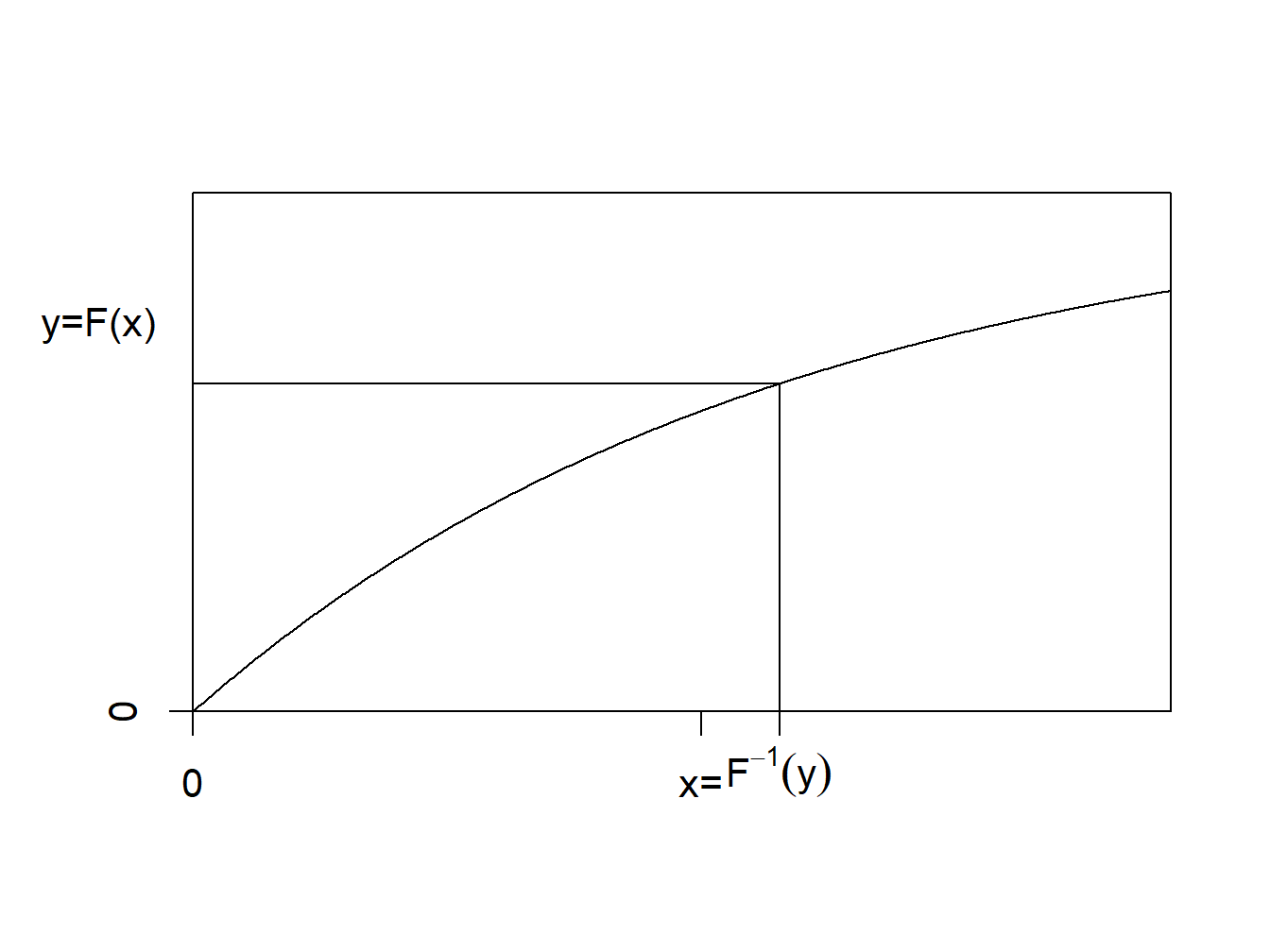
Figure 6.1: Inverse of a Distribution Function
The inverse transform result is available when the underlying random variable is continuous, discrete or a mixture. Here is a series of examples to illustrate its scope of applications.
Exponential Distribution Example. Suppose that we would like to generate observations from an exponential distribution with scale parameter \(\theta\) so that \(F(x) = 1 - e^{-x/\theta}\). To compute the inverse transform, we can use the following steps: \[\begin{aligned} y = F(x) &\Leftrightarrow y = 1-e^{-x/\theta} \\ &\Leftrightarrow -\theta \ln(1-y) = x = F^{-1}(y) .\end{aligned}\] Thus, if \(U\) has a uniform (0,1) distribution, then \(X = -\theta \ln(1-U)\) has an exponential distribution with parameter \(\theta\).
Some Numbers. Take \(\theta = 10\) and generate three random numbers to get
| \(U\) | 0.26321364 | 0.196884752 | 0.897884218 |
| \(X = -10\ln(1-U)\) | 1.32658423 | 0.952221285 | 9.909071325 |
Pareto Distribution Example. Suppose that we would like to generate observations from a Pareto distribution with parameters \(\alpha\) and \(\theta\) so that \(F(x) = 1 - \left(\frac{\theta}{x+\theta} \right)^{\alpha}\). To compute the inverse transform, we can use the following steps: \[\begin{aligned} y = F(x) &\Leftrightarrow 1-y = \left(\frac{\theta}{x+\theta} \right)^{\alpha} \\ &\Leftrightarrow \left(1-y\right)^{-1/\alpha} = \frac{x+\theta}{\theta} = \frac{x}{\theta} +1 \\ &\Leftrightarrow \theta \left((1-y)^{-1/\alpha} - 1\right) = x = F^{-1}(y) .\end{aligned}\] Thus, \(X = \theta \left((1-U)^{-1/\alpha} - 1\right)\) has a Pareto distribution with parameters \(\alpha\) and \(\theta\).
Inverse Transform Justification. Why does the random variable \(X = F^{-1}(U)\) have a distribution function “\(F\)”?
This is easy to establish in the continuous case. Because \(U\) is a Uniform random variable on (0,1), we know that \(\Pr(U \le y) = y\), for \(0 \le y \le 1\). Thus, \[\begin{aligned} \Pr(X \le x) &= \Pr(F^{-1}(U) \le x) \\ &= \Pr(F(F^{-1}(U)) \le F(x)) \\ &= \Pr(U \le F(x)) = F(x)\end{aligned}\] as required. The key step is that $ F(F^{-1}(u)) = u$ for each \(u\), which is clearly true when \(F\) is strictly increasing.
Bernoulli Distribution Example. Suppose that we wish to simulate random variables from a Bernoulli distribution with parameter \(p=0.85\). A graph of the cumulative distribution function shows that the quantile function can be written as
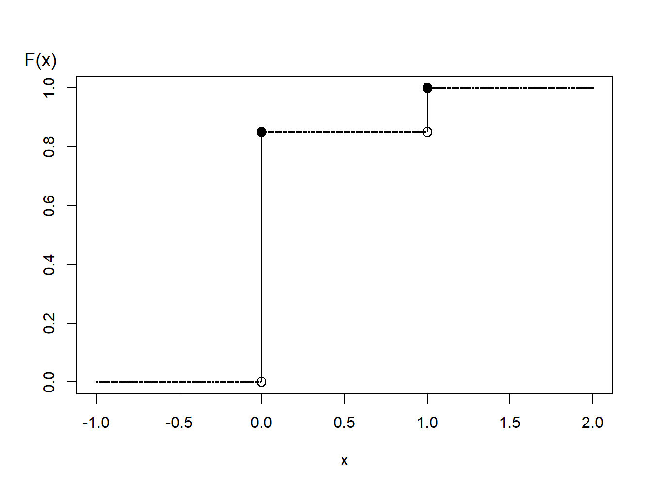
Figure 6.2: Distribution Function of a Binary Random Variable
\[\begin{aligned} F^{-1}(y) = \left\{ \begin{array}{cc} 0 & 0<y \leq 0.85 \\ 1 & 0.85 < y \leq 1.0 . \end{array} \right.\end{aligned}\]
Thus, with the inverse transform we may define \[\begin{aligned} X = \left\{ \begin{array}{cc} 0 & 0<U \leq 0.85 \\ 1 & 0.85 < U \leq 1.0 \end{array} \right.\end{aligned}\] Some Numbers. Generate three random numbers to get
| \(U\) | 0.26321364 | 0.196884752 | 0.897884218 |
| \(X =F^{-1}(U)\) | 0 | 0 | 1 |
Discrete Distribution Example. Consider the time of a machine failure in the first five years. The distribution of failure times is given as:
| Time (\(x\)) | 1 | 2 | 3 | 4 | 5 |
| probability | 0.1 | 0.2 | 0.1 | 0.4 | 0.2 |
| \(F(x)\) | 0.1 | 0.3 | 0.4 | 0.8 | 1.0 |
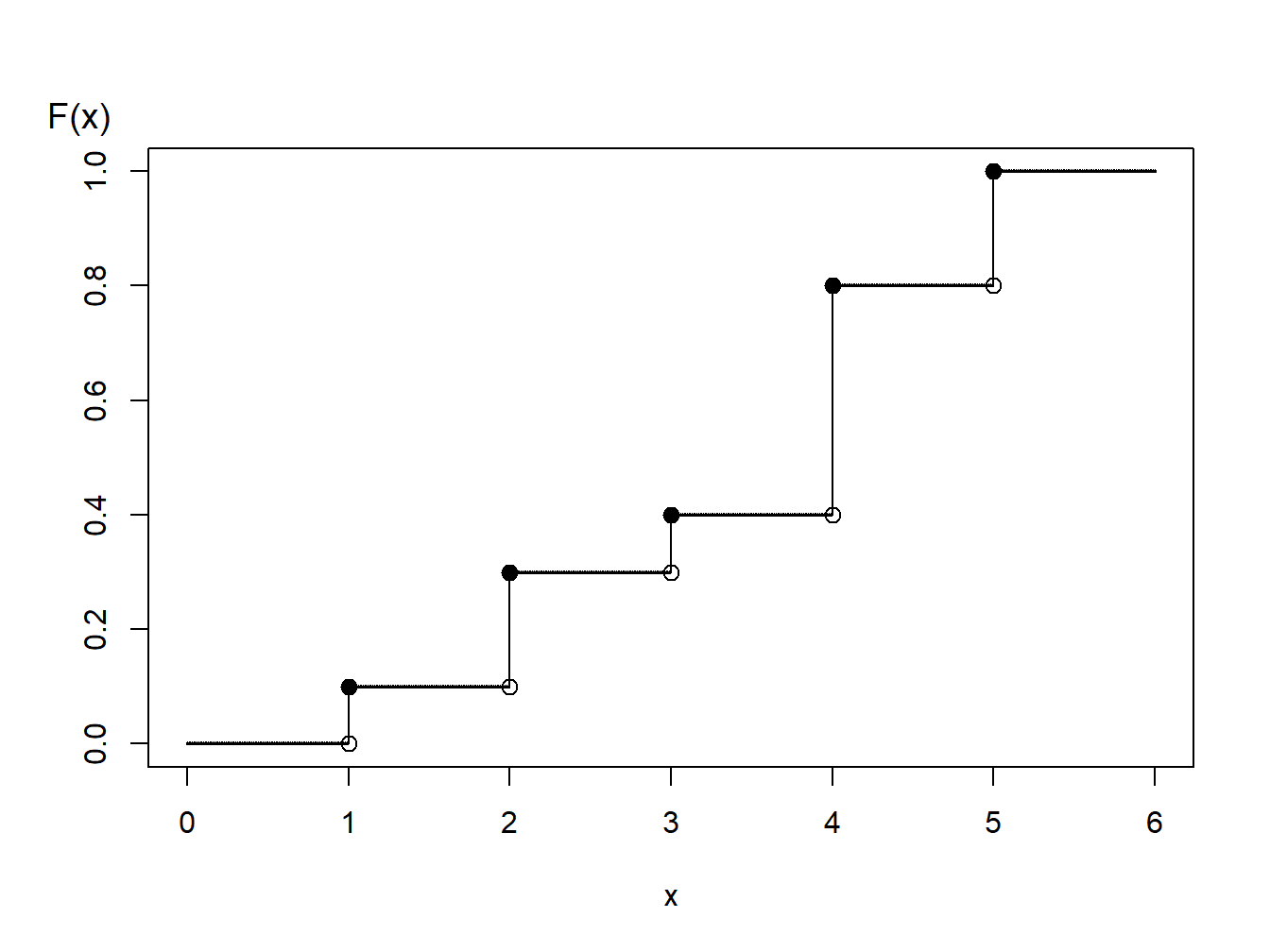
Figure 6.3: Distribution Function of a Discrete Random Variable
Using the graph of the distribution function, with the inverse transform we may define \[\begin{aligned} X = \left\{ \begin{array}{cc} 1 & 0<U \leq 0.1 \\ 2 & 0.1 < U \leq 0.3\\ 3 & 0.3 < U \leq 0.4\\ 4 & 0.4 < U \leq 0.8 \\ 5 & 0.8 < U \leq 1.0 . \end{array} \right.\end{aligned}\]
For general discrete random variables there may not be an ordering of outcomes. For example, a person could own one of five types of life insurance products and we might use the following algorithm to generate random outcomes:
\[\begin{aligned} X = \left\{ \begin{array}{cc} \textrm{whole life} & 0<U \leq 0.1 \\ \textrm{endowment} & 0.1 < U \leq 0.3\\ \textrm{term life} & 0.3 < U \leq 0.4\\ \textrm{universal life} & 0.4 < U \leq 0.8 \\ \textrm{variable life} & 0.8 < U \leq 1.0 . \end{array} \right.\end{aligned}\]
Another analyst may use an alternative procedure such as:
\[\begin{aligned} X = \left\{ \begin{array}{cc} \textrm{whole life} & 0.9<U<1.0 \\ \textrm{endowment} & 0.7 \leq U < 0.9\\ \textrm{term life} & 0.6 \leq U < 0.7\\ \textrm{universal life} & 0.2 \leq U < 0.6 \\ \textrm{variable life} & 0 \leq U < 0.2 . \end{array} \right.\end{aligned}\]
Both algorithms produce (in the long-run) the same probabilities, e.g., \(\Pr(\textrm{whole life})=0.1\), and so forth. So, neither is incorrect. You should be aware that there is “more than one way to skin a cat.” (What an old expression!) Similarly, you could use an alterative algorithm for ordered outcomes (such as failure times 1, 2, 3, 4, or 5, above).
Mixed Distribution Example. Consider a random variable that is 0 with probability 70% and is exponentially distributed with parameter \(\theta= 10,000\) with probability 30%. In practice, this might correspond to a 70% chance of having no insurance claims and a 30% chance of a claim - if a claim occurs, then it is exponentially distributed. The distribution function is given as
\[\begin{aligned} F(y) = \left\{ \begin{array}{cc} 0 & x<0 \\ 1 - 0.3 \exp(-x/10000) & x \ge 0 . \end{array} \right.\end{aligned}\]
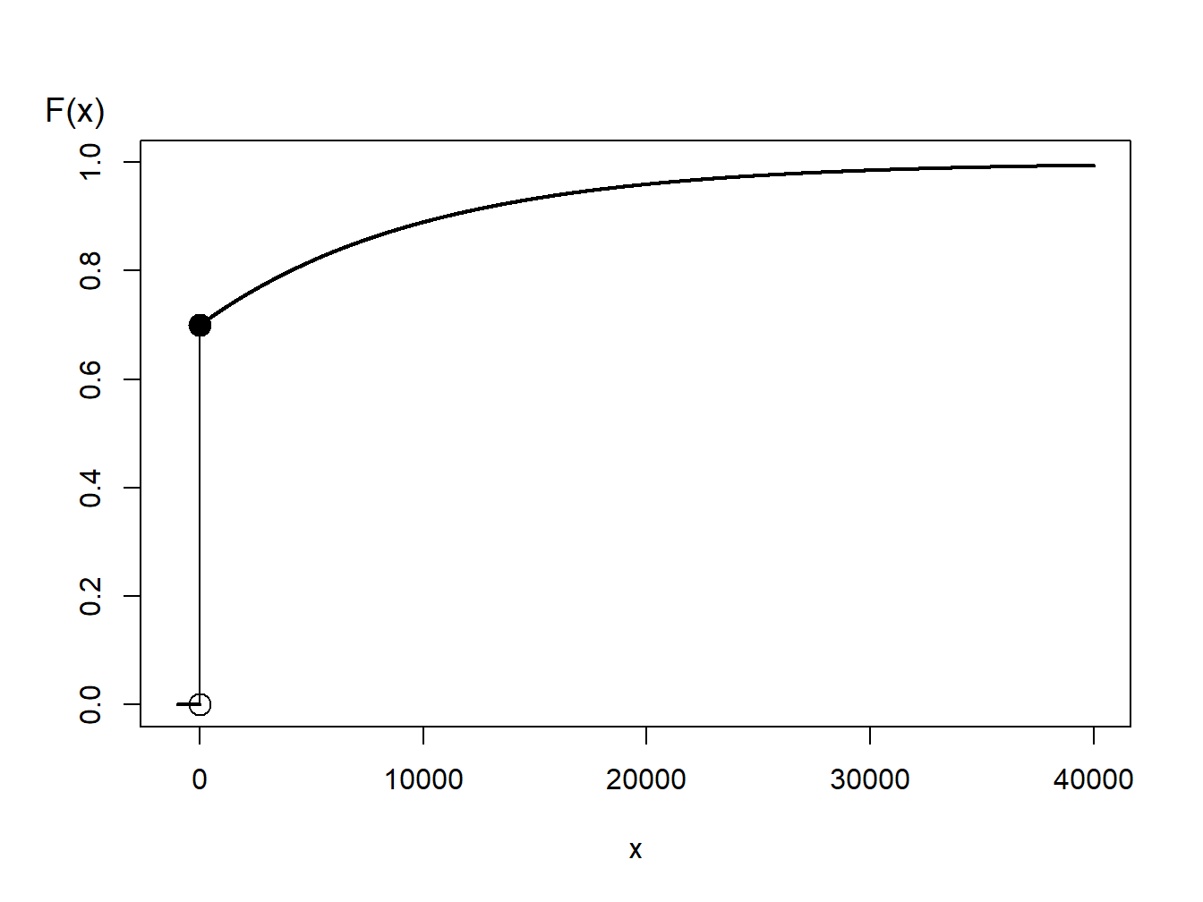
Figure 6.4: Distribution Function of a Hybrid Random Variable
From the graph, we can see that the inverse transform for generating random variables with this distribution function is
\[\begin{aligned} X = F^{-1}(U) = \left\{ \begin{array}{cc} 0 & 0< U \leq 0.7 \\ -1000 \ln (\frac{1-U}{0.3}) & 0.7 < U < 1 . \end{array} \right.\end{aligned}\]
As you have seen, for the discrete and mixed random variables, the key is to draw a graph of the distribution function that allows you to visualize potential values of the inverse function.
6.3 How Many Simulated Values?
There are many topics to be described in the study of simulation (and fortunately many good sources to help you). The best way to appreciate simulation is to experience it. One topic that inevitably comes up is the number of simulated trials needed to rid yourself of sampling variability so that you may focus on patterns of interest.
How many simulated values are recommended? 100? 1,000,000? We can use the central limit theorem to respond to this question. Suppose that we wish to use simulation to calculate \(\mathrm{E~}h(X)\), where \(h(\cdot)\) is some known function. Then, based on \(R\) simulations (replications), we get $ X_1,,X_R$. From this simulated sample, we calculate a sample average \[\overline{h}_R=\frac{1}{R}\sum_{i=1}^{R} h(X_i)\] and a sample standard deviation \[s_{h,R}^2 = \frac{1}{R} \sum_{i=1}^{R}\left( h(X_i) -\overline{h}_R \right) ^2.\] So, \(\overline{h}_R\) is your best estimate of \(\mathrm{E~}h(X)\) and \(s_{h,R}^2\) provides an indication of the uncertainty of your estimate. As one criterion for your confidence in the result, suppose that you wish to be within 1% of the mean with 95% certainty. According to the central limit theorem, your estimate should be approximately normally distributed. Thus, you should continue your simulation until \[\frac{.01\overline{h}_R}{s_{h,R}/\sqrt{R}}\geq 1.96\] or equivalently \[R \geq 38,416\frac{s_{h,R}^2}{\overline{h}_R^2}.\] This criterion is a direct application of the approximate normality (recall that 1.96 is the 97.5th percentile of the standard normal curve). Note that \(\overline{h}_R\) and \(s_{h,R}\) are not known in advance, so you will have to come up with estimates as you go (sequentially), either by doing a little pilot study in advance or by interrupting your procedure intermittently to see if the criterion is satisfied.