Chapter 2 Frequency Modeling

Chapter Preview. A primary focus for insurers is estimating the magnitude of aggregate claims it must bear under its insurance contracts. Aggregate claims are affected by both the frequency of insured events and the severity of the insured event. Decomposing aggregate claims into these two components, which each warrant significant attention, is essential for analysis and pricing. This chapter discusses frequency distributions, measures, and parameter estimation techniques.

2.1 Frequency Distributions

2.1.1 How Frequency Augments Severity Information

2.1.1.1 Basic Terminology

We use claim to denote the indemnification upon the occurrence of an insured event. Some authors use claim and loss interchangeably, while others think of loss as the amount suffered by the insured whereas claim is the amount paid by the insurer. Frequency represents how often an insured event occurs, typically within a policy contract. Here, we focus on count random variables that represent the number of claims, that is, how frequently an event occurs within a policy term. Severity denotes the amount, or size, of each payment for an insured event. In future chapters, the aggregate model, which combines frequency models with severity models, is examined.

2.1.1.2 The Importance of Frequency

Recall from Chapter 1 that setting the price of an insurance good can be a complex problem. In manufacturing, the cost of a good is (relatively) known. In other financial service areas, market prices are available. In insurance, we can generalize the price setting as follows: start with an expected cost. Add “margins” to account for the product’s riskiness, expenses incurred in servicing the product, and a profit/surplus allowance for the insurer.

That expected cost for insurance can be defined as the expected number of claims times the expected amount per claim, that is, expected frequency times severity. The focus on claim count allows the insurer to consider those factors which directly affect the occurrence of a loss, thereby potentially generating a claim. The frequency process can then be modeled.

2.1.1.3 Why Examine Frequency Information

Insurers and other stakeholders, including governmental organizations, have various motivations for gathering and maintaining frequency datasets.

• Contractual - In insurance contracts, it is common for particular deductibles and policy limits to be listed and invoked for each occurrence of an insured event. Correspondingly, the claim count data generated would indicate the number of claims which meet these criteria, offering a unique claim frequency measure. Extending this, models of total insured losses would need to account for deductibles and policy limits for each insured event.
• Behavioral - In considering factors that influence loss frequency, the risk-taking and risk-reducing behavior of individuals and companies should be considered. Explanatory (rating) variables can have different effects on models of how often an event occurs in contrast to the size of the event.
  • In healthcare, the decision to utilize healthcare by individuals, and minimize such healthcare utilization through preventive care and wellness measures, is related primarily to his or her personal characteristics. The cost per user is determined by those personal characteristics, the medical condition, potential treatment measures, and decisions made by the healthcare provider (such as the physician) and the patient. While there is overlap in those factors and how they affect total healthcare costs, attention can be focused on those separate drivers of healthcare visit frequency and healthcare cost severity.
  • In personal lines, prior claims history is an important underwriting factor. It is common to use an indicator of whether or not the insured had a claim within a certain time period prior to the contract.
  • In homeowners insurance, in modeling potential loss frequency, the insurer could consider loss prevention measures that the homeowner has adopted, such as visible security systems. Separately, when modeling loss severity, the insurer would examine those factors that affect repair and replacement costs.
• Databases. Many insurers keep separate data files that suggest developing separate frequency and severity models. For example, a policyholder file is established when a policy is written. This file records much underwriting information about the insured(s), such as age, gender, and prior claims experience, policy information such as coverage, deductibles and limitations, as well as the insurance claims event. A separate file, known as the “claims” file, records details of the claim against the insurer, including the amount. (There may also be a ``payments’’ file that records the timing of the payments although we shall not deal with that here.) This recording process makes it natural for insurers to model the frequency and severity as separate processes.
• Regulatory and Administrative Insurance is a highly regulated and monitored industry, given its importance in providing financial security to individuals and companies facing risk. As part of its duties, regulators routinely require the reporting of claims numbers as well as amounts. This may be due to the fact that there can be alternative definitions of an ``amount,’’ e.g., paid versus incurred, and there is less potential error when reporting claim numbers. This continual monitoring helps ensure financial stability of these insurance companies.

2.2 Basic Frequency Distributions

In this section, we will introduce the distributions that are commonly used in actuarial practice to model count data. The claim count random variable is denoted by \(N\); by its very nature it assumes only non-negative integral values. Hence the distributions below are all discrete distributions supported on the set of non-negative integers (\(\mathbb{Z}^+\)).

2.2.1 Foundations

Since \(N\) is a discrete random variable taking values in \(\mathbb{Z}^+\), the most natural full description of its distribution is through the specification of the probabilities with which it assumes each of the non-negative integral values. This leads us to the concept of the probability mass function (pmf) of \(N\), denoted as \(p_N(\cdot)\) and defined as follows: \[\begin{equation} p_N(k)=\Pr(N=k), \quad \hbox{for } k=0,1,\ldots \end{equation}\] We note that there are alternate complete descriptions, or characterizations, of the distribution of \(N\); for example, the distribution function of \(N\) denoted by \(F_N(\cdot)\) and defined below is another such: \[\begin{equation} F_N(x):=\begin{cases} \sum\limits_{k=0}^{\lfloor x \rfloor } \Pr(N=k), &x\geq 0;\\ 0, & \hbox{otherwise}. \end{cases} \end{equation}\]

In the above, \(\lfloor \cdot \rfloor\) denotes the floor function; \(\lfloor x \rfloor\) denotes the greatest integer less than or equal to \(x\). We note that the survival function of \(N\), denoted by \(S_N(\cdot)\), is defined as the ones’-complement of \(F_N(\cdot)\), i.e. \(S_N(\cdot):=1-F_N(\cdot)\). Clearly, the latter is another characterization of the distribution of \(N\).

Often one is interested in quantifying a certain aspect of the distribution and not in its complete description. This is particularly useful when comparing distributions. A center of location of the distribution is one such aspect, and there are many different measures that are commonly used to quantify it. Of these, the mean is the most popular; the mean of \(N\), denoted by \(\mu_N\)², is defined as

\[\begin{equation} \mu_N=\sum_{k=0}^\infty kp_N(k). \end{equation}\] We note that \(\mu_N\) is the expected value of the random variable \(N\), i.e. \(\mu_N=\mathrm{E}~N\). This leads to a general class of measures, the **moments*8 of the distribution; the \(r\)-th moment of \(N\), for \(r> 0\), is defined as \(\mathrm{E}{N^r}\) and denoted by \(\mu_N'(r)\). Hence, for \(r>0\), we have
\[\begin{equation} \mu_N(r)= \mathrm{E}{N^r}= \sum_{k=0}^\infty k^r p_N(k). \end{equation}\]

We note that \(\mu_N'(\cdot)\) is a well-defined non-decreasing function taking values in \([0,\infty)\), as \(\Pr(N\in\mathbb{Z}^+)=1\); also, note that \(\mu_N=\mu_N'(1)\).

Another basic aspect of a distribution is its dispersion, and of the various measures of dispersion studied in the literature, the standard deviation is the most popular. Towards defining it, we first define the variance of \(N\), denoted by \(\mathrm{Var}~N\), as \(\mathrm{Var}~N:=\mathrm{E}{(N-\mu_N)^2}\) when \(\mu_N\) is finite. By basic properties of the expected value of a random variable, we see that \(\mathrm{Var}~N:=\mathrm{E}~{N^2}-(\mathrm{E}~N)^2\). The standard deviation of \(N\), denoted by \(\sigma_N\), is defined as the square-root of \(\mathrm{Var}~N\). Note that the latter is well-defined as \(\mathrm{Var}~N\), by its definition as the average squared deviation from the mean, is non-negative; \(\mathrm{Var}~N\) is denoted by \(\sigma_N^2\). Note that these two measures take values in \([0,\infty)\).

2.2.2 Moment and Probability Generating Functions

Now we will introduce two generating functions that are found to be useful when working with count variables. Recall that the moment generating function (mgf) of \(N\), denoted as \(M_N(\cdot)\), is defined as \[ M_N(t) = \mathrm{E}~{e^{tN}} = \sum^{\infty}_{k=0} ~e^{tk}~ p_N(k), \quad t\in \mathbb{R}. \] We note that while \(M_N(\cdot)\) is well defined as it is the expectation of a non-negative random variable (\(e^{tN}\)), though it can assume the value \(\infty\). Note that for a count random variable, \(M_N(\cdot)\) is finite valued on \((-\infty,0]\) with \(M_N(0)=1\). The following theorem, whose proof can be found in (Billingsley 2008) (pages 285-6), encapsulates the reason for its name of moment generating functions.

Theorem 2.1 Let \(N\) be a count random variable such that \(\mathrm{E}~{e^{t^\ast N}}\) is finite for some \(t^\ast>0\). We have the following:

All moment of \(N\) are finite, i.e. \[ \mathrm{E}{N^r}<\infty, \quad r\geq 0. \] The mgf can be used to generate its moments as follows: \[ \left.\frac{{\rm d}^m}{{\rm d}t^m} M_N(t)\right\vert_{t=0}=\mathrm{E}{N^m}, \quad m\geq 1. \] The mgf \(M_N(\cdot)\) characterizes the distribution; in other words it uniquely specifies the distribution.

Another reason that the mgf is very useful as a tool is that for two independent random variables \(X\) and \(Y\), with their mgfs existing in a neighborhood of \(0\), the mgf of \(X+Y\) is the product of their respective mgfs.

A related generating function to the mgf is called the probability generating function (pgf), and is a useful tool for random variables taking values in \(\mathbb{Z}^+\). For a random variable \(N\), by \(P_N(\cdot)\) we denote its pgf and we define it as follows: \[\begin{equation} P_N(s):=\mathrm{E}~{s^N}, \quad s\geq 0. \end{equation}\]

It is straightforward to see that if the mgf \(M_N(\cdot)\) exists on \((-\infty,t^\ast)\) then \[ P_N(s)=M_N(\log(s)), \quad s<e^{t^\ast}. \] Moreover, if the pgf exists on an interval \([0,s^\ast)\) with \(s^\ast>1\), then the mgf \(M_N(\cdot)\) exists on \((-\infty,\log(s^\ast))\), and hence uniquely specifies the distribution of \(N\) by Theorem 2.1. The following result for pgf is an analog of Theorem 2.1, and in particular justifies its name.

Theorem 2.2 Let \(N\) be a count random variable such that \(\mathrm{E}~{(s^{\ast})^N}\) is finite for some \(s^\ast>1\). We have the following:

All moment of \(N\) are finite, i.e. \[ \mathrm{E}~{N^r}<\infty, \quad r\geq 0. \] The pmf of \(N\) can be derived from the pgf as follows: \[ p_N(m)=\begin{cases} P_N(0), &m=0;\cr &\cr \left(\frac{1}{m!}\right) \left.\frac{{\rm d}^m}{{\rm d}s^m} P_N(s)\right\vert_{s=0}\;, &m\geq 1.\cr \end{cases} \] The factorial moments of \(N\) can be derived as follows: \[ \left.\frac{{\rm d}^m}{{\rm d}s^m} P_N(s)\right\vert_{s=1}=\mathrm{E}~{\prod\limits_{i=0}^{m-1} (N-i)}, \quad m\geq 1. \] The pgf \(P_N(\cdot)\) characterizes the distribution; in other words it uniquely specifies the distribution.

2.2.3 Important Frequency Distributions

In this sub-section we will study three important frequency distributions used in statistics, namely the binomial, the negative binomial and the Poisson distributions. In the following, a risk denotes a unit covered by insurance. A risk could be an individual, a building, a company, or some other identifier for which insurance coverage is provided. For context, imagine an insurance data set containing the number of claims by risk or stratified in some other manner. The above mentioned distributions also happen to be the most commonly used in insurance practice for various reasons, some of which we mention below.

• These distributions can be motivated by natural random experiments which are good approximations to real life processes from which many insurance data arise. Hence, not surprisingly, they together offer a reasonable fit to many insurance data sets of interest. The appropriateness of a particular distribution for the set of data can be determined using standard statistical methodologies, as we discuss later in this chapter.
• They provide a rich enough basis for generating other distributions that even better approximate or well cater to more real situations of interest to us.
  • The three distributions are either one-parameter or two-parameter distributions. In fitting to data, a parameter is assigned a particular value. The set of these distributions can be enlarged to their convex hulls by treating the parameter(s) as a random variable (or vector) with its own probability distribution, with this larger set of distributions offering greater flexibility. A simple example that is better addressed by such an enlargement is a portfolio of claims generated by insureds belonging to many different risk classes.
  • In insurance data, we may observe either a marginal or inordinate number of zeros, i.e. zero claims by risk. When fitting to the data, a frequency distribution in its standard specification often fails to reasonably account for this occurrence. The natural modification of the above three distributions, however, accommodate this phenomenon well towards offering a better fit.
  • In insurance we are interested in total claims paid, whose distribution results from compounding the fitted frequency distribution with a severity distribution. These three distributions have properties that make it easy to work with the resulting aggregate severity distribution.

2.2.3.1 Binomial Distribution

We begin with the binomial distribution which arises from any finite sequence of identical and independent experiments with binary outcomes. The most canonical of such experiments is the (biased or unbiased) coin tossing experiment with the outcome being heads or tails. So if \(N\) denotes the number of heads in a sequence of \(m\) independent coin tossing experiments with an identical coin which turns heads up with probability \(q\), then the distribution of \(N\) is called the binomial distribution with parameters \((m,q)\), with \(m\) a positive integer and \(q\in[0,1]\). Note that when \(q=0\) (resp., \(q=1\)) then the distribution is degenerate with \(N=0\) (resp., \(N=m\)) with probability \(1\). Clearly, its support when \(q\in(0,1)\) equals \(\{0,1,\ldots,m\}\) with pmf given by³

\[\begin{equation*} p_k:= \binom{m}{k} q^k (1-q)^{m-k}, \quad k=0,\ldots,m. \end{equation*}\]

The reason for its name is that the pmf takes values among the terms that arise from the binomial expansion of \((q +(1-q))^m\). This realization then leads to the the following expression for the pgf of the binomial distribution: \[ P(z):= \sum_{k=0}^m z^k \binom{m}{k} q^k (1-q)^{m-k} = \sum_{k=0}^m \binom{m}{k} (zq)^k (1-q)^{m-k} = (qz+(1-q))^m = (1+q(z-1))^m. \] Note that the above expression for the pgf confirms the fact that the binomial distribution is the \(m\)-convolution of the Bernoulli distribution, which is the binomial distribution with \(m=1\) and pgf \((1+q(z-1))\). Also, note that the mgf of the binomial distribution is given by \((1+q(e^t-1))^m\).

The central moments of the binomial distribution can be found in a few different ways. To emphasize the key property that it is a \(m\)-convolution of the Bernoulli distribution, we derive below the moments using this property. We begin by observing that the Bernoulli distribution with parameter \(q\) assigns probability of \(q\) and \(1-q\) to \(1\) and \(0\), respectively. So its mean equals \(q\) (\(=0\times (1-q) + 1\times q\)); note that its raw second moment equals its mean as \(N^2=N\) with probability \(1\). Using these two facts we see that the variance equals \(q(1-q)\). Moving on to the binomial distribution with parameters \(m\) and \(q\), using the fact that it is the \(m\)-convolution of the Bernoulli distribution, we write \(N\) as the sum of \(N_1,\ldots,N_m\), where \(N_i\) are iid Bernoulli variates. Now using the moments of Bernoulli and linearity of the expectation, we see that \[ \mathrm{E}~{N}=\mathrm{E}~{\sum_{i=1}^m N_i} = \sum_{i=1}^m ~\mathrm{E}~{N_i} = mq. \] Also, using the fact that the variance of the sum of independent random variables is the sum of their variances, we see that
\[ \mathrm{Var}~{N}=\mathrm{Var}~\left({\sum_{i=1}^m N_i}\right)=\sum_{i=1}^m \mathrm{Var}~{N_i} = mq(1-q). \] Alternate derivations of the above moments are suggested in the exercises. One important observation, especially from the point of view of applications, is that the mean is greater than the variance unless \(q=0\).

2.2.3.2 Poisson Distribution

After the binomial distribution, the Poisson distribution (named after the French polymath Sim'eon Denis Poisson) is probably the most well known of discrete distributions. This is partly due to the fact that it arises naturally as the distribution of the count of the random occurrences of a type of event in a certain time period, if the rate of occurrences of such events is a constant. Relatedly, it also arises as the asymptotic limit of the binomial distribution with \(m\rightarrow \infty\) and \(mq\rightarrow \lambda\).

The Poisson distribution is parametrized by a single parameter usually denoted by \(\lambda\) which takes values in \((0,\infty)\). Its pmf is given by \[ p_k = \frac{e^{-\lambda}\lambda^k}{k!}, k=0,1,\ldots \] It is easy to check that the above specifies a pmf as the terms are clearly non-negative, and that they sum to one follows from the infinite Taylor series expansion of \(e^\lambda\). More generally, we can derive its pgf, \(P(\cdot)\), as follows: \[ P(z):= \sum_{k=0}^\infty p_k z^k = \sum_{k=0}^\infty \frac{e^{-\lambda}\lambda^kz^k}{k!} = e^{-\lambda} e^{\lambda z} = e^{\lambda(z-1)}, \forall z\in\mathbb{R}. \] From the above, we derive its mgf as follows: \[ M(t)=P(e^t)=e^{\lambda(e^t-1)}, t\in \mathbb{R}. \] Towards deriving its mean, we note that for the Poisson distribution \[ kp_k=\begin{cases} 0, &k=0;\cr \lambda p_{k-1}, &k\geq1; \end{cases} \] this can be checked easily. In particular, this implies that \[ \mathrm{E}~{N}=\sum_{k\geq 0} k~p_k =\lambda\sum_{k\geq 1} p_{k-1} = \lambda\sum_{j\geq 0} p_{j} =\lambda. \] In fact, more generally, using either a generalization of the above or using Theorem 2.2, we see that \[ \mathrm{E}{\prod\limits_{i=0}^{m-1} (N-i)}=\left.\frac{{\rm d}^m}{{\rm d}s^m} P_N(s)\right\vert_{s=1}=\lambda^m, \quad m\geq 1. \] This, in particular, implies that \[ \mathrm{Var}~{N}=\mathrm{E}~{N^2}-(\mathrm{E}~{N})^2 = \mathrm{E}~{N(N-1)}+\mathrm{E}~{N}-(\mathrm{E}~{N})^2=\lambda^2+\lambda-\lambda^2=\lambda. \] Note that interestingly for the Poisson distribution \(\mathrm{Var}~{N}=\mathrm{E}~{N}\).

2.2.3.3 Negative binomial Distribution

The third important count distribution is the negative binomial distribution. Recall that the binomial distribution arose as the distribution of the number of successes in \(m\) independent repetition of an experiment with binary outcomes. If we instead consider the number of successes until we observe the \(r\)-th failure in independent repetitions of an experiment with binary outcomes, then its distribution is a negative binomial distribution. A particular case, when \(r=1\), is the geometric distribution. In the following we will allow the parameter \(r\) to be any positive real, and unfortunately when \(r\) in not an integer the above random experiment would not be applicable. To then motivate the distribution more generally, and in the process explain its name, we recall the binomial series, i.e. \[ (1+x)^s= 1 + s x + \frac{s(s-1)}{2!}x^2 + \ldots..., \quad s\in\mathbb{R}; \vert x \vert<1. \] If we define \(\binom{s}{k}\), the generalized binomial coefficient, by \[ \binom{s}{k}=\frac{s(s-1)\cdots(s-k+1)}{k!}, \] then we have \[ (1+x)^s= \sum_{k=0}^{\infty} \binom{s}{k} x^k, \quad s\in\mathbb{R}; \vert x \vert<1. \] If we let \(s=-r\), then we see that the above yields \[ (1-x)^{-r}= 1 + r x + \frac{(r+1)r}{2!}x^2 + \ldots...= \sum_{k=0}^\infty \binom{r+k-1}{k} x^k, \quad r\in\mathbb{R}; \vert x \vert<1. \] This implies that if we define \(p_k\) as \[ p_k = \binom{k+r-1}{k} \left(\frac{1}{1+\beta}\right)^r \left(\frac{\beta}{1+\beta}\right)^k, \quad k=0,1,\ldots \] for \(r>0\) and \(\beta>=0\), then it defines a valid pmf. Such defined distribution is called the negative binomial distribution with parameters \((r,\beta)\) with \(r>0\) and \(\beta\geq 0\). Moreover, the binomial series also implies that the pgf of this distribution is given by \[ \begin{aligned} P(z) &= (1-\beta(z-1))^{-r}, \quad \vert z \vert \leq 1+\frac{1}{\beta}, \beta\geq0. \end{aligned} \] The above implies that the mgf is given by \[ \begin{aligned} M(t) &= (1-\beta(e^t-1))^{-r}, \quad t \leq \log\left(1+\frac{1}{\beta}\right), \beta\geq0. \end{aligned} \] We derive its moments using Theorem 2.1 as follows:

\[\begin{eqnarray*} \mathrm{E}~{N}&=&M'(0)= \left. r\beta e^t (1-\beta(e^t-1))^{-r-1}\right\vert_{t=0}=r\beta;\\ \mathrm{E}~{N^2}&=&M''(0)= \left.\left[ r\beta e^t (1-\beta(e^t-1))^{-r-1} + r(r+1)\beta^2 e^{2t} (1-\beta(e^t-1))^{-r-2}\right]\right\vert_{t=0}\\ &=&r\beta(1+\beta)+r^2\beta^2;\\ \hbox{and }\mathrm{E}{N}&=&\mathrm{E}{N^2}-(\mathrm{E}{N})^2=r\beta(1+\beta)+r^2\beta^2-r^2\beta^2=r\beta(1+\beta) \end{eqnarray*}\]

We note that when \(\beta>0\), we have \(\mathrm{Var}~{N} >\mathrm{E}~{N}\). In other words, this distribution is overdispersed (relative to the Poisson); similarly, when \(q>0\) the binomial distribution is said to be underdispersed (relative to the Poisson).

Finally, we observe that the Poisson distribution also emerges as a limit of negative binomial distributions. Towards establishing this, let \(\beta_r\) be such that as \(r\) approaches infinity \(r\beta_r\) approaches \(\lambda>0\). Then we see that the mgfs of negative binomial distributions with parameters \((r,\beta_r)\) satisfies \[ \lim_{r\rightarrow 0} (1-\beta_r(e^t-1))^{-r}=\exp\{\lambda(e^t-1)\}, \] with the right hand side of the above equation being the mgf of the Poisson distribution with parameter \(\lambda\)⁴

2.3 The (a, b, 0) Class

In the previous section we studied three distributions, namely the binomial, the Poisson and the negative binomial distributions. In the case of the Poisson, to derive its mean we used the the fact that \[ kp_k=\lambda p_{k-1}, \quad k\geq 1, \] which can be expressed equivalently as \[ \frac{p_k}{p_{k-1}}=\frac{\lambda}{k}, \quad k\geq 1. \] Interestingly, we can similarly show that for the binomial distribution \[ \frac{p_k}{p_{k-1}}=\frac{-q}{1-q}+\left(\frac{(m+1)q}{1-q}\right)\frac{1}{k}, \quad k=1,\ldots,m, \] and that for the negative binomial distribution \[ \frac{p_k}{p_{k-1}}=\frac{\beta}{1+\beta}+\left(\frac{(r-1)\beta}{1+\beta}\right)\frac{1}{k}, \quad k\geq 1. \] The above relationships are all of the form \[\begin{equation} \frac{p_k}{p_{k-1}}=a+\frac{b}{k}, \quad k\geq 1; \tag{2.1} \end{equation}\]

this raises the question if there are any other distributions which satisfy this seemingly general recurrence relation.

To begin with let \(a<0\). In this case as \((a+b/k)\rightarrow a<0\) as \(k\rightarrow \infty\), and the ratio on the left is non-negative, it follows that if \(a<0\) then \(b\) should satisfy \(b=-ka\), for some \(k\geq 1\). Any such pair \((a,b)\) can be written as \[ \left(\frac{-q}{1-q},\frac{(m+1)q}{1-q}\right), \quad q\in(0,1), m\geq 1; \] note that the case \(a<0\) with \(a+b=0\) yields the degenerate at \(0\) distribution which is the binomial distribution with \(q=0\) and arbitrary \(m\geq 1\).

In the case of \(a=0\), again by non-negativity of the ratio \(p_k/p_{k-1}\), we have \(b\geq 0\). If \(b=0\) the distribution is degenerate at \(0\), which is a binomial with \(q=0\) or a Poisson distribution with \(\lambda=0\) or a negative binomial distribution with \(\beta=0\). If \(b>0\), then clearly such a distribution is a Poisson distribution with mean (i.e. \(\lambda\)) equal to \(b\).

In the case of \(a>0\), again by non-negativity of the ratio \(p_k/p_{k-1}\), we have \(a+b/k\geq 0\) for all \(k\geq 1\). The most stringent of these is the inequality \(a+b\geq 0\). Note that \(a+b=0\) again results in degeneracy at \(0\); excluding this case we have \(a+b>0\) or equivalently \(b=(r-1)a\) with \(r>0\). Some algebra easily yields the following expression for \(p_k\): \[ p_k = \binom{k+r-1}{k} p_0 a^k, \quad k=1,2,\ldots. \] The above series converges for \(a<1\) when \(r>0\), with the sum given by \(p_0*((1-a)^{(-r)}-1)\). Hence, equating the latter to \(1-p_0\) we get \(p_0=(1-a)^{(-r)}\). So in this case the pair \((a,b)\) is of the form \((a,(r-1)a)\), for \(r>0\) and \(0<a<1\); since a equivalent parametrization is \((\beta/(1+\beta),(r-1)\beta/(1+\beta))\), for \(r>0\) and \(0<\beta\), we see from above that such distributions are negative binomial distributions.

From the above development we see that not only does the recurrence (2.1) tie these three distributions together, but also it characterizes them. For this reason these three distributions are collectively referred to in the actuarial literature as \((a,b,0)\) class of distributions, with \(0\) referring to the starting point of the recurrence. Note that the value of \(p_0\) is implied by \((a,b)\) since the probabilities have to sum to one. Of course, (2.1) as a recurrence relation for \(p_k\) makes the computation of the pmf efficient by removing redundancies. Later, we will see that it does so even in the case of compound distributions with the frequency distribution belonging to the \((a,b,0)\) class - this fact is the more important motivating reason to study these three distribution from this viewpoint.

Example 2.3.1. A discrete probability distribution has the following properties \[ \begin{aligned} p_k&=c\left( 1+\frac{2}{k}\right) p_{k-1} \:\:\: k=1,2,3,\ldots\\ p_1&= \frac{9}{256} \end{aligned} \] Determine the expected value of this discrete random variable.

Show Example Solution

Solution: Since the pmf satisfies the \((a,b,0)\) recurrence relation we know that the underlying distribution is one among the binomial, Poisson and negative binomial distributions. Since the ratio of the parameters (i.e. \(b/a\)) equals \(2\), we know that it is negative binomial and that \(r=3\). Moreover, since for a negative binomial \(p_1=r(1+\beta)^{-(r+1)}\beta\), we have \(\beta=3\). Finally, since the mean of a negative binomial is \(r\beta\) we have the mean of the given distribution equals \(9\).

---

2.4 Estimating Frequency Distributions

2.4.1 Parameter estimation

In Section 2.2 we introduced three distributions of importance in modeling various types of count data arising from insurance. Let us now suppose that we have a set of count data to which we wish to fit a distribution, and that we have determined that one of these \((a,b,0)\) distributions is more appropriate than the others. Since each one of these forms a class of distributions if we allow its parameter(s) to take any permissible value, there remains the task of determining the best value of the parameter(s) for the data at hand. This is a statistical point estimation problem, and in parametric inference problems the statistical inference paradigm of maximum likelihood usually yields efficient estimators. In this section we will describe this paradigm and derive the maximum likelihood estimators (mles).

Let us suppose that we observe the iid random variables \(X_1,X_2,\ldots,X_n\) from a distribution with pmf \(p_\theta\), where \(\theta\) is an unknown value in \(\Theta\subseteq \mathbb{R}^d\). For example, in the case of the Poisson distribution \[ p_\theta(x)=e^{-\theta}\frac{\theta^x}{x!}, \quad x=0,1,\ldots, \] with \(\Theta=(0,\infty)\). In the case of the binomial distribution we have \[ p_\theta(x)=\binom{m}{x} q^x(1-q)^{m-x}, \quad x=0,1,\ldots,m, \] with \(\theta:=(m,q)\in \{0,1,2,\ldots\}\times(0,1]\). Let us suppose that the observations are \(x_1,\ldots,x_n\); in this case the probability of observing this sample from \(p_\theta\) equals \[ \prod_{i=1}^n p_\theta(x_i). \] The above, denoted by \(L(\theta)\), viewed as a function of \(\theta\) is called the likelihood. Note that we suppressed its dependence on the data, to emphasize that we are viewing it as a function of the parameter. For example, in the case of the Poisson distribution we have \[ L(\lambda)=e^{-n\lambda} \lambda^{\sum_{i=1}^n x_i} \left(\prod_{i=1}^n x_i!\right)^{-1}; \] in the case of the binomial distribution we have \[ L(m,q)=\left(\prod_{i=1}^n \binom{m}{x_i}\right) q^{\sum_{i=1}^n x_i} (1-q)^{nm-\sum_{i=1}^n x_i} . \] The maximum likelihood estimator (mle) for \(\theta\) is any maximizer of the likelihood; in a sense the mle chooses the parameter value that best explains the observed observations. Consider a sample of size \(3\) from a Bernoulli distribution (binomial with \(m=1\)) with values \(0,1,0\). The likelihood in this case is easily checked to equal \[ L(q)=q(1-q)^2, \] and the plot of the likelihood is given in Figure 2.1. As shown in the plot, the maximum value of the likelihood equals \(4/27\) and is attained at \(q=1/3\), and hence the mle for \(q\) is \(1/3\) for the given sample. In this case one can resort to algebra to show that \[ q(1-q)^2=\left(q-\frac{1}{3}\right)^2\left(q-\frac{4}{3}\right)+\frac{4}{27}, \]

and conclude that the maximum equals \(4/27\), and is attained at \(q=1/3\) (using the fact that the first term is non-positive in the interval \([0,1]\)). But as is apparent, this way of deriving the mle using algebra does not generalize. In general, one resorts to calculus to derive the mle - note that for some likelihoods one may have to resort to other optimization methods, especially when the likelihood has many local extrema. It is customary to equivalently maximize the logarithm of the likelihood⁵ \(L(\cdot)\), denoted by \(l(\cdot)\), and look at the set of zeros of its first derivative⁶ \(l'(\cdot)\). In the case of the above likelihood, \(l(q)=\log(q)+2\log(1-q)\), and

\[ l'(q):=\frac{\rm d}{{\rm d}q}l(q)=\frac{1}{q}-\frac{2}{1-q}. \] The unique zero of \(l'(\cdot)\) equals \(1/3\), and since \(l''(\cdot)\) is negative, we have \(1/3\) is the unique maximizer of the likelihood and hence its mle.

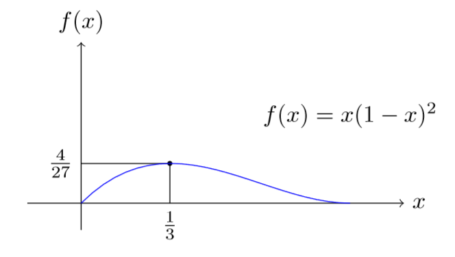
Figure 2.1: Likelihood of a \((0,1,0)\) \(3\)-sample from Bernoulli

2.4.2 Frequency Distributions MLE

In the following, we derive the mle for the three members of the \((a,b,0)\) class. We begin by summarizing the discussion above. In the setting of observing iid random variables \(X_1,X_2,\ldots,X_n\) from a distribution with pmf \(p_\theta\), where \(\theta\) is an unknown value in \(\Theta\subseteq \mathbb{R}^d\), the likelihood \(L(\cdot)\), a function on \(\Theta\) is defined as \[ L(\theta):=\prod_{i=1}^n p_\theta(x_i), \] where \(x_1,\ldots,x_n\) are the observed values. The maximum likelihood estimator (mle) of \(\theta\), denoted as \(\hat{\theta}_{\rm MLE}\) is a function which maps the observations to an element of the set of maximizers of \(L(\cdot)\), namely \[ \{\theta \vert L(\theta)=\max_{\eta\in\Theta}L(\eta)\}. \] Note the above set is a function of the observations, even though this dependence is not made explicit. In the case of the three distributions that we will study, and quite generally, the above set is a singleton with probability tending to one (with increasing sample size). In other words, for many commonly used distributions and when the sample size is large, the mle is uniquely defined with high probability.

In the following, we will assume that we have observed \(n\) iid random variables \(X_1,X_2,\ldots,X_n\) from the distribution under consideration, even though the parametric value is unknown. Also, \(x_1,x_2,\ldots,x_n\) will denote the observed values. We note that in the case of count data, and data from discrete distributions in general, the likelihood can alternately be represented as \[ L(\theta):=\prod_{k\geq 0} \left(p_\theta(k)\right)^{m_k}, \] where \[ m_k:= \left\vert \{i\vert x_i=k, 1\leq i \leq n\} \right\vert=\sum_{i= 1}^n I(x_i=k), \quad k\geq 0. \] Note that this is an information loss-less transformation of the data. For large \(n\) it leads to compression of the data in the sense of sufficiency. Below, we present expressions for the mle in terms of \(\{m_k\}_{k\geq 1}\) as well.

MLE - Poisson Distribution: In this case, as noted above, the likelihood is given by \[ L(\lambda)=\left(\prod_{i=1}^n x_i!\right)^{-1}e^{-n\lambda}\lambda^{\sum_{i=1}^n x_i}, \] which implies that \[ l(\lambda)= -\sum_{i=1}^n \log(x_i!) -n\lambda +\log(\lambda) \cdot \sum_{i=1}^n x_i, \] and \[ l'(\lambda)= -n +\frac{1}{\lambda}\sum_{i=1}^n x_i. \] Since \(l''< 0\) if \(\sum_{i=1}^n x_i>0\), the maximum is attained at the sample mean. In the contrary, the maximum is attained at the least possible parameter value, that is the mle equals zero. Hence, we have
\[ \hat{\lambda}_{\rm MLE} = \frac{1}{n}\sum_{i=1}^n X_i. \] Note that the sample mean can be computed also as \[ \frac{1}{n} \sum_{k\geq 1} km_k. \] It is noteworthy that in the case of the Poisson, the exact distribution of \(\hat{\lambda}_{\rm MLE}\) is available in closed form - it is a scaled Poisson - when the underlying distribution is a Poisson. This is so as the sum of independent Poisson random variables is a Poisson as well. Of course, for large sample size one can use the ordinary Central Limit Theorem (CLT) to derive a normal approximation. Note that the latter approximation holds even if the underlying distribution is any distribution with a finite second moment.

MLE - Binomial distribution: Unlike the case of the Poisson distribution, the parameter space in the case of the binomial is \(2\)-dimensional. Hence the optimization problem is a bit more challenging. We begin by observing that the likelihood is given by \[ L(m,q)= \left(\prod_{i=1}^n \binom{m}{x_i}\right) q^{\sum_{i=1}^n x_i} (1-q)^{nm-\sum_{i=1}^n x_i}, \] and the log-likelihood by \[ l(m,q)= \sum_{i=1}^n \log\left(\binom{m}{x_i}\right) + \left({\sum_{i=1}^n x_i}\right)\log(q)+ \left({nm-\sum_{i=1}^n x_i}\right)\log(1-q). \] Note that since \(m\) takes only non-negative integral values, we cannot use multivariate calculus to find the optimal values. Nevertheless, we can use single variable calculus to show that \[\begin{equation} \hat{q}_{\rm MLE}\times \hat{m}_{\rm MLE}= \frac{1}{n}\sum_{i=1}^n X_i. \tag{2.2} \end{equation}\] Towards this we note that for a fixed value of \(m\), \[ \frac{\delta}{\delta q} l(m,q) = \left({\sum_{i=1}^n x_i}\right)\frac{1}{q}- \left({nm-\sum_{i=1}^n x_i}\right)\frac{1}{1-q}, \] and that \[ \frac{\delta^2}{\delta q^2} l(m,q) = -\left[\left({\sum_{i=1}^n x_i}\right)\frac{1}{q^2} + \left({nm-\sum_{i=1}^n x_i}\right)\frac{1}{(1-q)^2}\right]\leq 0. \] The above implies that for any fixed value of \(m\), the maximizing value of \(q\) satisfies \[ mq=\frac{1}{n}\sum_{i=1}^n X_i, \] and hence we establish equation (2.2). The above reduces the task to the search for \(\hat{m}_{\rm MLE}\), which is member of the set of the maximizers of \[\begin{equation} L\left(m,\frac{1}{nm}\sum_{i=1}^n x_i\right). \tag{2.3} \end{equation}\]

Note the likelihood would be zero for values of \(m\) smaller than \(\max\limits_{1\leq i \leq n}x_i\), and hence \[ \hat{m}_{\rm MLE}\geq \max_{1\leq i \leq n}x_i. \] Towards specifying an algorithm to compute \(\hat{m}_{\rm MLE}\), we first point out that for some data sets \(\hat{m}_{\rm MLE}\) could equal \(\infty\), indicating that a Poisson distribution would render a better fit than any binomial distribution. This is so as the binomial distribution with parameters \((m,\overline{x}/m)\) approaches the Poisson distribution with parameter \(\overline{x}\) with \(m\) approaching infinity. The fact that some data sets will prefer a Poisson distribution should not be surprising since in the above sense the set of Poisson distribution is on the boundary of the set of binomial distributions.

Interestingly, in (Olkin, Petkau, and Zidek 1981) they show that if the sample mean is less than or equal to the sample variance then \(\hat{m}_{\rm MLE}=\infty\); otherwise, there exists a finite \(m\) that maximizes equation (2.3). In Figure 2.2 below we display the plot of \(L\left(m,\frac{1}{nm}\sum_{i=1}^n x_i\right)\) for three different samples of size \(5\); they differ only in the value of the sample maximum. The first sample of \((2,2,2,4,5)\) has the ratio of sample mean to sample variance greater than \(1\) (\(1.875\)), the second sample of \((2,2,2,4,6)\) has the ratio equal to \(1.25\) which is closer to \(1\), and the third sample of \((2,2,2,4,7)\) has the ratio less than \(1\) (\(0.885\)). For these three samples, as shown in Figure 2.2, \(\hat{m}_{\rm MLE}\) equals \(7\), \(18\) and \(\infty\), respectively. Note that the limiting value of \(L\left(m,\frac{1}{nm}\sum_{i=1}^n x_i\right)\) as \(m\) approaches infinity equals \[\begin{equation} \left(\prod_{i=1}^n x_i! \right)^{-1} \exp\left\{-\sum_{i=1}^n x_i\right\} \overline{x}^{n\overline{x}}. \tag{2.4} \end{equation}\]

Also, note that Figure 2.2 shows that the mle of \(m\) is non-robust, i.e. changes in a small proportion of the data set can cause large changes in the estimator.

The above discussion suggests the following simple algorithm:

• Step 1. If the sample mean is less than or equal to the sample variance, \(\hat{m}_{MLE}=\infty\). The mle suggested distribution is a Poisson distribution with \(\hat{\lambda}=\overline{x}\).
• Step 2. If the sample mean is greater than the sample variance, then compute \(L(m,\overline{x}/m)\) for \(m\) values greater than or equal to the sample maximum until \(L(m,\overline{x}/m)\) is close to the value of the Poisson likelihood given in . The value of \(m\) that corresponds to the maximum value of \(L(m,\overline{x}/m)\) among those computed equals \(\hat{m}_{MLE}\).

We note that if the underlying distribution is the binomial distribution with parameters \((m,q)\) (with \(q>0\)) then \(\hat{m}_{MLE}\) will equal \(m\) for large sample sizes. Also, \(\hat{q}_{MLE}\) will have an asymptotically normal distribution and converge with probability one to \(q\).

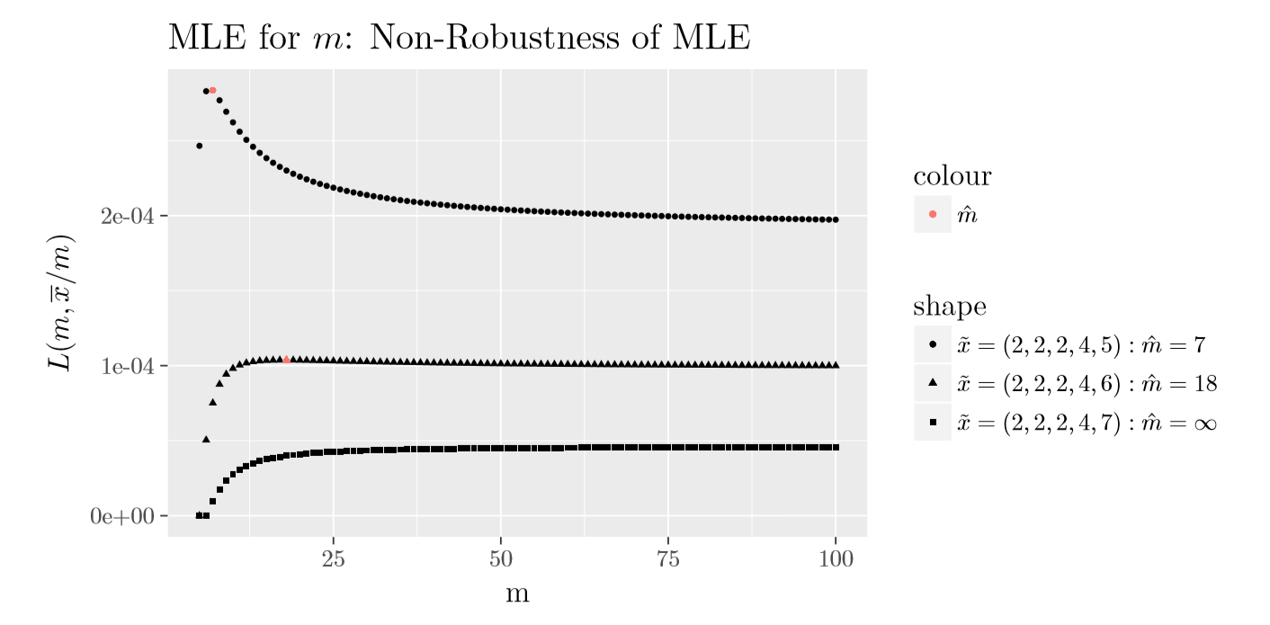
Figure 2.2: Plot of \(L(m,\overline{x}/m)\) for binomial distribution

MLE - Negative binomial Distribution: The case of the negative binomial distribution is similar to that of the binomial distribution in the sense that we have two parameters and the MLEs are not be available in closed form. A difference between them is that unlike the binomial parameter \(m\) which takes positive integral values, the parameter \(r\) of the negative binomial can assume any positive real value. This makes the optimization problem a tad more complex. We begin by observing that the likelihood can be expressed in the following form: \[ L(r,\beta)=\left(\prod_{i=1}^n \binom{r+x_i-1}{x_i}\right) (1+\beta)^{-n(r+\overline{x})} \beta^{n\overline{x}}. \] The above implies that log-likelihood is given by \[ l(r,\beta)=\sum_{i=1}^n \log\binom{r+x_i-1}{x_i} -n(r+\overline{x}) \log(1+\beta) +n\overline{x}\log\beta, \] and hence \[ \frac{\delta}{\delta\beta} l(r,\beta) = -\frac{n(r+\overline{x})}{1+\beta} + \frac{n\overline{x}}{\beta}. \] Equating the above to zero, we get \[ \hat{r}_{MLE}\times \hat{\beta}_{MLE} = \overline{x}. \] The above reduces the two dimensional optimization problem to a one-dimensional problem - we need to maximize \[ l(r,\overline{x}/r)=\sum_{i=1}^n \log\binom{r+x_i-1}{x_i} -n(r+\overline{x}) \log(1+\overline{x}/r) +n\overline{x}\log(\overline{x}/r), \] with respect to \(r\), with the maximizing \(r\) being its mle and \(\hat{\beta}_{MLE}=\overline{x}/\hat{r}_{MLE}\). In (Levin, Reeds, and others 1977) it is show that if the sample variance is greater than the sample mean then there exists a unique \(r>0\) that maximizes \(l(r,\overline{x}/r)\) and hence a unique MLE for \(r\) and \(\beta\). Also, they show that if \(\hat{\sigma}^2\leq \overline{x}\), then the negative binomial likelihood will be dominated by the Poisson likelihood with \(\hat{\lambda}=\overline{x}\) - in other words, a Poisson distribution offers a better fit to the data. The guarantee in the case of \(\hat{\sigma}^2>\hat{\mu}\) permits us to use any algorithm to maximize \(l(r,\overline{x}/r)\). Towards an alternate method of computing the likelihood, we note that \[ l(r,\overline{x}/r)=\sum_{i=1}^n \sum_{j=1}^{x_i}\log(r-1+j) - \sum_{i=1}^n\log(x_i!) - n(r+\overline{x}) \log(r+\overline{x}) + nr\log(r) + n\overline{x}\log(\overline{x}), \] which yields \[ \left(\frac{1}{n}\right)\frac{\delta}{\delta r}l(r,\overline{x}/r)=\left(\frac{1}{n}\right)\sum_{i=1}^n \sum_{j=1}^{x_i}\frac{1}{r-1+j} - \log(r+\overline{x}) + \log(r). \] We note that, in the above expressions, the inner sum equals zero if \(x_i=0\). The mle for \(r\) is a zero of the last expression, and hence a root finding algorithm can be used to compute it. Also, we have \[ \left(\frac{1}{n}\right)\frac{\delta^2}{\delta r^2}l(r,\overline{x}/r)=\frac{\overline{x}}{r(r+\overline{x})}-\left(\frac{1}{n}\right)\sum_{i=1}^n \sum_{j=1}^{x_i}\frac{1}{(r-1+j)^2}. \] A simple but quickly converging iterative root finding algorithm is the Newton’s method, which incidentally the Babylonians are believed to have used for computing square roots. Applying the Newton’s method to our problem results in the following algorithm:
Step i. Choose an approximate solution, say \(r_0\). Set \(k\) to \(0\).
Step ii. Define \(r_{k+1}\) as \[ r_{k+1}:= r_k - \frac{\left(\frac{1}{n}\right)\sum_{i=1}^n \sum_{j=1}^{x_i}\frac{1}{r_k-1+j} - \log(r_k+\overline{x}) + \log(r_k)}{\frac{\overline{x}}{r_k(r_k+\overline{x})}-\left(\frac{1}{n}\right)\sum_{i=1}^n \sum_{j=1}^{x_i}\frac{1}{(r_k-1+j)^2}} \]
Step iii. If \(r_{k+1}\sim r_k\), then report \(r_{k+1}\) as MLE; else increment \(k\) by \(1\) and repeat Step ii.

For example, we simulated a \(5\) sample of \(41, 49, 40, 27, 23\) from the negative binomial with parameters \(r=10\) and \(\beta=5\). Choosing the starting value of \(r\) such that \[ r\beta=\hat{\mu} \quad \hbox{and} \quad r\beta(1+\beta)=\hat{\sigma}^2 \] leads to the starting value of \(23.14286\). The iterates of \(r\) from the Newton’s method are \[ 21.39627, 21.60287, 21.60647, 21.60647; \] the rapid convergence seen above is typical of the Newton’s method. Hence in this example, \(\hat{r}_{MLE}\sim21.60647\) and \(\hat{\beta}_{MLE}=8.3308\)

R Implementation of Newton’s Method - Negative binomial MLE for \(r\)

Show R Code

Newton<-function(x,abserr){
mu<-mean(x);
sigma2<-mean(x^2)-mu^2;
r<-mu^2/(sigma2-mu);
b<-TRUE;
iter<-0;
while (b) {
tr<-r;
m1<-mean(c(x[x==0],sapply(x[x>0],function(z){sum(1/(tr:(tr-1+z)))})));
m2<-mean(c(x[x==0],sapply(x[x>0],function(z){sum(1/(tr:(tr-1+z))^2)})));
r<-tr-(m1-log(1+mu/tr))/(mu/(tr*(tr+mu))-m2);
b<-!(abs(tr-r)<abserr);
iter<-iter+1;
}
c(r,iter)
}

---

To summarize our discussion of mle for the \((a,b,0)\) class of distributions, in Figure 2.3 below we plot the maximum value of the Poisson likelihood, \(L(m,\overline{x}/m)\) for the binomial, and \(L(r,\overline{x}/r)\) for the negative binomial, for the three samples of size \(5\) given in Table 2.1. The data was constructed to cover the three orderings of the sample mean and variance. As show in the Figure 2.3, and supported by theory, if \(\hat{\mu}<\hat{\sigma}^2\) then the negative binomial will result in a higher maximum likelihood value; if \(\hat{\mu}=\hat{\sigma}^2\) the Poisson will have the highest likelihood value; and finally in the case that \(\hat{\mu}>\hat{\sigma}^2\) the binomial will give a better fit than the others. So before fitting a frequency data with an \((a,b,0,)\) distribution, it is best to start with examining the ordering of \(\hat{\mu}\) and \(\hat{\sigma}^2\). We again emphasize that the Poisson is on the boundary of the negative binomial and binomial distributions. So in the case that \(\hat{\mu}\geq\hat{\sigma}^2\) (\(\hat{\mu}\leq\hat{\sigma}^2\), resp.) the Poisson will yield a better fit than the negative binomial (binomial, resp.), which will also be indicated by \(\hat{r}=\infty\) (\(\hat{m}=\infty\), resp.).

\[\begin{matrix} \begin{array}{c|c|c} \hline \text{Data} & \text{Mean }(\hat{\mu}) & \text{Variance }(\hat{\sigma}^2) \\ \hline (2,3,6,8,9) & 5.60 & 7.44 \\ (2,5,6,8,9) & 6 & 6\\ (4,7,8,10,11) & 8 & 6\\\hline \end{array} \end{matrix}\]

Table 2.1 : Three Samples of Size \(5\)

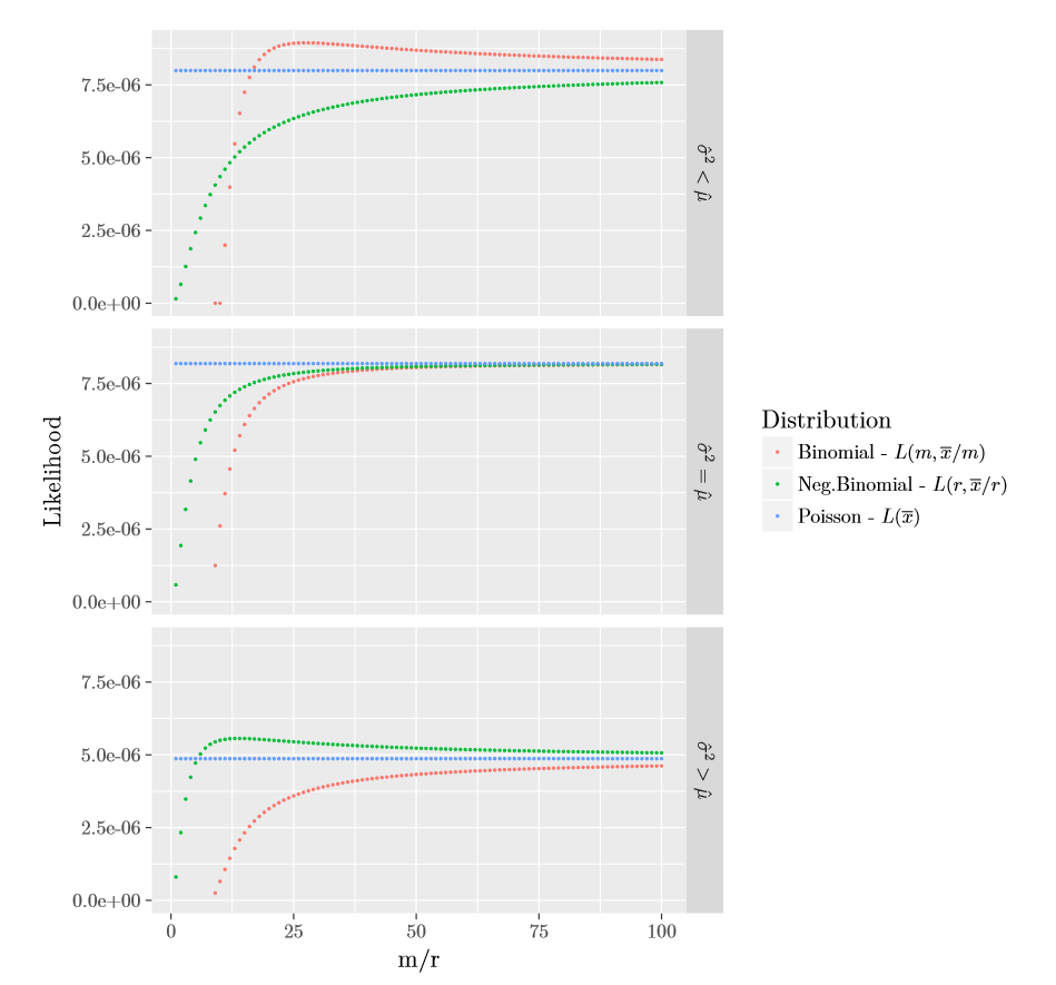
Figure 2.3: Plot of \((a,b,0)\) Partially Maximized Likelihoods

2.5 Other Frequency Distributions

In the above we discussed three distributions with supports contained in the set of non-negative integers, which well cater to many insurance applications. Moreover, typically by allowing the parameters to be a function of known (to the insurer) explanatory variables such as age, sex, geographic location (territory), and so forth, these distributions allow us to explain claim probabilities in terms of these variables. The field of statistical study that studies such models is known as regression analysis - it is an important topic of actuarial interest that we will not pursue in this book; see (Edward W Frees 2009).

There are clearly infinitely many other count distributions, and more importantly the above distributions by themselves do not cater to all practical needs. In particular, one feature of some insurance data is that the proportion of zero counts can be out of place with the proportion of other counts to be explainable by the above distributions. In the following we modify the above distributions to allow for arbitrary probability for zero count irrespective of the assignment of relative probabilities for the other counts. Another feature of a data set which is naturally comprised of homogeneous subsets is that while the above distributions may provide good fits to each subset, they may fail to do so to the whole data set. Later we naturally extend the \((a,b,0)\) distributions to be able to cater to, in particular, such data sets.

2.5.1 Zero Truncation or Modification

Let us suppose that we are looking at auto insurance policies which appear in a database of auto claims made in a certain period. If one is to study the number of claims that these policies have made during this period, then clearly the distribution has to assign a probability of zero to the count variable assuming the value zero. In other words, by restricting attention to count data from policies in the database of claims, we have in a sense zero-truncated the count data of all policies. In personal lines (like auto), policyholders may not want to report that first claim because of fear that it may increase future insurance rates - this behavior will inflate the proportion of zero counts. Examples such as the latter modify the proportion of zero counts. Interestingly, natural modifications of the three distributions considered above are able to provide good fits to zero-modified/truncated data sets arising in insurance.

In the below we modify the probability assigned to zero count by the \((a,b,0)\) class while maintaining the relative probabilities assigned to non-zero counts - zero modification. Note that since the \((a,b,0)\) class of distribution satisfies the recurrence (2.1), maintaining relative probabilities of non-zero counts implies that recurrence (2.1) is satisfied for \(k\geq 2\). This leads to the definition of the following class of distributions.

Definition. A count distribution is a member of the \((a, b, 1)\) class if for some constants \(a\) and \(b\) the probabilities \(p_k\) satisfy \[\begin{equation} \frac{p_k}{p_{k-1}}=a+\frac{b}{k},\quad k\geq 2. \tag{2.5} \end{equation}\]

Note that since the recursion starts with \(p_1\), and not \(p_0\), we refer to this super-class of \((a,b,0)\) distributions by \((a,b,1)\). To understand this class, recall that each valid pair of values for \(a\) and \(b\) of the \((a,b,0)\) class corresponds to a unique vector of probabilities \(\{p_k\}_{k\geq 0}\). If we now look at the probability vector \(\{\tilde{p}_k\}_{k\geq 0}\) given by \[ \tilde{p}_k= \frac{1-\tilde{p}_0}{1-p_0}\cdot p_k, \quad k\geq 1, \] where \(\tilde{p}_0\in[0,1)\) is arbitrarily chosen, then since the relative probabilities for positive values according to \(\{p_k\}_{k\geq 0}\) and \(\{\tilde{p}_k\}_{k\geq 0}\) are the same, we have \(\{\tilde{p}_k\}_{k\geq 0}\) satisfies recurrence (2.5). This, in particular, shows that the class of \((a,b,1)\) distributions is strictly wider than that of \((a,b,0)\).

In the above, we started with a pair of values for \(a\) and \(b\) that led to a valid \((a,b,0)\) distribution, and then looked at the \((a,b,1)\) distributions that corresponded to this \((a,b,0)\) distribution. We will now argue that the \((a,b,1)\) class allows for a larger set of permissible values for \(a\) and \(b\) than the \((a,b,0)\) class. Recall from Section 2.3 that in the case of \(a<0\) we did not use the fact that the recurrence (2.1) started at \(k=1\), and hence the set of pairs \((a,b)\) with \(a<0\) that are permissible for the \((a,b,0)\) class is identical to those that are permissible for the \((a,b,1)\) class. The same conclusion is easily drawn for pairs with \(a=0\). In the case that \(a>0\), instead of the constraint \(a+b>0\) for the \((a,b,0)\) class we now have the weaker constraint of \(a+b/2>0\) for the \((a,b,1)\) class. With the parametrization \(b=(r-1)a\) as used in Section 2.3, instead of \(r>0\) we now have the weaker constraint of \(r>-1\). In particular, we see that while zero modifying a \((a,b,0)\) distribution leads to a distribution in the \((a,b,1)\) class, the conclusion does not hold in the other direction.

Zero modification of a count distribution \(F\) such that it assigns zero probability to zero count is called a zero truncation of \(F\). Hence, the zero truncated version of probabilities \(\{p_k\}_{k\geq 0}\) is given by \[ \tilde{p}_k=\begin{cases} 0, & k=0;\\ \frac{p_k}{1-p_0}, & k\geq 1. \end{cases} \]

In particular, we have that a zero modification of a count distribution \(\{p_k\}_{k\geq 0}\), denoted by \(\{p^M_k\}_{k\geq 0}\), can be written as a convex combination of the degenerate distribution at \(0\) and the zero truncation of \(\{p_k\}_{k\geq 0}\), denoted by \(\{p^T_k\}_{k\geq 0}\). That is we have \[ p^M_k= p^M_0 \cdot \delta_{0}(k) + (1-p^M_0) \cdot p^T_k, \quad k\geq 0. \]

Example 2.5.1. Zero Truncated/Modified Poisson. Consider a Poisson distribution with parameter \(\lambda=2\). Calculate \(p_k, k=0,1,2,3\), for the usual (unmodified), truncated and a modified version with \((p_0^M=0.6)\).

Show Example Solution

Solution. For the Poisson distribution as a member of the (\(a,b\),0) class, we have \(a=0\) and \(b=\lambda=2\). Thus, we may use the recursion \(p_k = \lambda p_{k-1}/k= 2 p_{k-1}/k\) for each type, after determining starting probabilities. The calculation of probabilities for \(k\leq 3\) is shown in Table 2.2.

\[\begin{matrix} \begin{array}{c|c|c|c} \hline k & p_k & p_k^T & p_k^M\\\hline 0 & p_0=e^{-\lambda}=0.135335 & 0 & 0.6\\\hline 1 & p_1=p_0(0+\frac{\lambda}{1})=0.27067 & \frac{p_1}{1-p_0}=0.313035 & \frac{1-p_0^M}{1-p_0}~p_1=0.125214\\\hline 2 & p_2=p_1\left( \frac{\lambda}{2}\right)=0.27067 & p_2^T=p_1^T\left(\frac{\lambda}{2}\right)=0.313035 & p_2^M=0.125214\\\hline 3 & p_3=p_2\left(\frac{\lambda}{3}\right)=0.180447 & p_3^T=p_2^T\left(\frac{\lambda}{3}\right)=0.208690 & p_3^M=p_2^M\left(\frac{\lambda}{3}\right)=0.083476\\\hline \end{array} \end{matrix}\]

Table 2.2 : Calculation of probabilities for \(k\leq 3\)

---

2.6 Mixture Distributions

In many applications, the underlying population consists of naturally defined sub-groups with some homogeneity within each sub-group. In such cases it is convenient to model the individual sub-groups, and in a ground-up manner model the whole population. As we shall see below, beyond the aesthetic appeal of the approach, it also extends the range of applications that can be catered to by standard parametric distributions.

Let \(k\) denote the number of defined sub-groups in a population, and let \(F_i\) denote the distribution of an observation drawn from the \(i\)-th subgroup. If we let \(\alpha_i\) denote the proportion of the population in the \(i\)-th subgroup, then the distribution of a randomly chosen observation from the population, denoted by \(F\), is given by \[\begin{equation} F(x)=\sum_{i=1}^n \alpha_i \cdot F_i(x). \tag{2.6} \end{equation}\]

The above expression can be seen as a direct application of Bayes theorem. As an example, consider a population of drivers split broadly into two sub-groups, those with less than \(5\)-years of driving experience and those with more than \(5\)-years experience. Let \(\alpha\) denote the proportion of drivers with less than \(5\) years experience, and \(F_{\leq 5}\) and \(F_{> 5}\) denote the distribution of the count of claims in a year for a driver in each group, respectively. Then the distribution of claim count of a randomly selected driver is given by \[ \alpha\cdot F_{\leq 5} + (1-\alpha)F_{> 5}. \]

An alternate definition of a mixture distribution is as follows. Let \(N_i\) be a random variable with distribution \(F_i\), \(i=1,\ldots, k\). Let \(I\) be a random variable taking values \(1,2,\ldots,k\) with probabilities \(\alpha_1,\ldots,\alpha_k\), respectively. Then the random variable \(N_I\) has a distribution given by equation (2.6)⁷.

In (2.6) we see that the distribution function is a convex combination of the component distribution functions. This result easily extends to the density function, the survival function, the raw moments, and the expectation as these are all linear functionals of the distribution function. We note that this is not true for central moments like the variance, and conditional measures like the hazard rate function. In the case of variance it is easily seen as \[ \mathrm{E}{N_I}=\mathrm{E}{\mathrm{E}{N_I\vert I}} + \mathrm{E}{\mathrm{E}{N_I|I}}=\sum_{i=1}^k \alpha_i \mathrm{E}{N_i} + \mathrm{E}{\mathrm{E}{N_I|I}}, \] and hence is not a convex function of the variances unless the group means are all equal.

Example 2.6.1. SOA Exam Question. In a certain town the number of common colds an individual will get in a year follows a Poisson distribution that depends on the individual’s age and smoking status. The distribution of the population and the mean number of colds are as follows:

\[\begin{matrix} \begin{array}{l|c|c} \hline & \text{Proportion of population} & \text{Mean number of colds}\\\hline \text{Children} & 0.3 & 3\\ \text{Adult Non-Smokers} & 0.6 & 1\\ \text{Adult Smokers} & 0.1 & 4\\\hline \end{array} \end{matrix}\]

Table 2.3 : The distribution of the population and the mean number of colds

1. Calculate the probability that a randomly drawn person has 3 common colds in a year.
2. Calculate the conditional probability that a person with exactly 3 common colds in a year is an adult smoker.

Show Example Solution

Solution.

1. Using development above, we can write the required probability as \(\Pr(N_I=3)\), with \(I\) denoting the group of the randomly selected individual with \(1,2\) and \(3\) signifying the groups Children, Adult Non-Smoker, and Adult Smoker, respectively. Now by conditioning we get \[ \Pr(N_I=3)=0.3\cdot\Pr(N_1=3)+0.6\cdot\Pr(N_2=3)+0.1\cdot\Pr(N_3=3), \] with \(N_1,N_2\) and \(N_3\) following Poisson distributions with means \(3,1\) and \(4\), respectively. Using the above, we get \(\Pr(N_I=3)\sim0.1235\)
2. The required probability can be written as \(\Pr(I=3\vert N_I=3)\), which equals \[ \Pr(I=3\vert N_I=3)=\frac{\Pr(I=3;N_3=3)}{\Pr(N_I=3)}\sim\frac{0.1 \times 0.1954}{0.1235}\sim 0.1581. \]

---

In the above example, the number of subgroups \(k\) was equal to three. In general, \(k\) can be any natural number, but when \(k\) is large it is parsimonious from a modeling point of view to take the following infinitely many subgroup approach. To motivate this approach, let the \(i\)-th subgroup be such that its component distribution \(F_i\) is given by \(G_{\tilde{\theta_i}}\), where \(G_\cdot\) is a parametric family of distributions with parameter space \(\Theta\subseteq \mathbb{R}^d\). With this assumption, the distribution function \(F\) of a randomly drawn observation from the population is given by \[ F(x)=\sum_{i=1}^k \alpha_i G_{\tilde{\theta_i}}(x),\quad \forall x\in\mathbb{R}. \] which can be alternately written as
\[ F(x)=\mathbf{R}{G_{\tilde{\vartheta}}(x)},\quad \forall x\in\mathbb{R}, \] where \(\tilde{\vartheta}\) takes values \(\tilde{\theta_i}\) with probability \(\alpha_i\), for \(i=1,\ldots,k\). The above makes it clear that when \(k\) is large, one could model the above by treating \(\tilde{\vartheta}\) as continuous random variable.

To illustrate this approach, suppose we have a population of drivers with the distribution of claims for an individual driver being distributed as a Poisson. Each person has their own (personal) expected number of claims \(\lambda\) - smaller values for good drivers, and larger values for others. There is a distribution of \(\lambda\) in the population; a popular and convenient choice for modeling this distribution is a gamma distribution with parameters \((\alpha, \theta)\). With these specifications it turns out that the resulting distribution of \(N\), the claims of a randomly chosen driver, is a negative binomial with parameters \((r=\alpha,\beta=\theta)\). This can be shown in many ways, but a straightforward argument is as follows:

\[\begin{align*} \Pr(N=k)&= \int_0^\infty \frac{e^{-\lambda}\lambda^k}{k!} \frac{\lambda^{\alpha-1}e^{-\lambda/\theta}}{\Gamma{(\alpha)}\theta^{\alpha}} {\rm d}\lambda = \frac{1}{k!\Gamma(\alpha)\theta^\alpha}\int_0^\infty \lambda^{\alpha+k-1}e^{-\lambda(1+1/\theta)}{\rm d}\lambda=\frac{\Gamma{(\alpha+k)}}{k!\Gamma(\alpha)\theta^\alpha(1+1/\theta)^{\alpha+k}} \\ &=\binom{\alpha+k-1}{k}\left(\frac{1}{1+\theta}\right)^\alpha\left(\frac{\theta}{1+\theta}\right)^k, \quad k=0,1,\ldots \end{align*}\]

It is worth mention that by considering mixtures of a parametric class of distributions we increase the richness of the class, resulting in the mixture class being able to cater well to more applications that the parametric class we started with. In the above case, this is seen as we have observed earlier that in a sense the Poisson distributions are on the boundary of negative binomial distributions and by mixing Poisson we get the interior distributions as well. Mixture modeling is a very important modeling technique in insurance applications, and later chapters will cover more aspects of this modeling technique.

Example 2.6.2. Suppose that \(N|\Lambda \sim\) Poisson\((\Lambda)\) and that \(\Lambda \sim\) gamma with mean of 1 and variance of 2. Determine the probability that \(N=1\).

Show Example Solution

Solution. For a gamma distribution with parameters \((\alpha, \theta)\), we have that the mean is \(\alpha \theta\) and the variance is \(\alpha \theta^2\). Using these expressions we have \[ \begin{aligned} \alpha &= \frac{1}{2} \text{ and } \theta =2. \end{aligned} \] Now, one can directly use the above result to conclude that \(N\) is distributed as a negative binomial with \(r = \alpha = \frac{1}{2}\) and \(\beta= \theta =2\). Thus \[ \begin{aligned} \Pr(N=1) &= \binom{1+r-1}{1}(\frac{1}{(1+\beta)^r})\left(\frac{\beta}{1+\beta}\right)^1 \\ &= \binom{1+\frac{1}{2}-1}{1}{\frac{1}{(1+2)^{1/2}}}\left(\frac{2}{1+2}\right)^1\\ &= \frac{1}{3^{3/2}} = 0.19245 . \end{aligned} \]

---

2.7 Goodness of Fit

In the above we have discussed three basic frequency distributions, along with their ways to enhance the reach of these classes through zero modification/truncation and by looking at mixtures of these distributions. Nevertheless, these classes still remain parametric and hence by their very nature a small subset of the class of all possible frequency distributions (i.e. the set of distributions on non-negative integers.) Hence, even though we have talked about methods for estimating the unknown parameters, the fitted distribution will not be a good representation of the underlying distribution if the latter is far from the class of distribution used for modeling. In fact, it can be shown that the mle estimate will converge to a value such that the fitted distribution will be a certain projection of the underlying distribution on the class of distributions used for modeling. Below we present one testing method - Pearson’s chi-square statistic - to check for the goodness of fit of the fitted distribution.

In \(1993\), a portfolio of \(n=7,483\) automobile insurance policies from a major Singaporean insurance company had the distribution of auto accidents per policyholder as given in Table 2.4.

\[\begin{matrix} \begin{array}{c|c|c|c|c|c|c} \hline \text{Count }(k) & 0 & 1 & 2 & 3 & 4 & \text{Total}\\ \hline \text{No. of Policies with }k\text{ accidents }(m_k) & 6,996 & 455 & 28 & 4 & 0 & 7483\\ \hline \end{array} \end{matrix}\]

Table 2.4 : Singaporean Automobile Accident Data

If we a fit a Poisson distribution, then the mle for \(\lambda\), the Poisson mean, is the sample mean which is given by \[ \overline{N} = \frac{0\cdot 6996 + 1 \cdot 455 + 2 \cdot 28 + 3 \cdot 4 + 4 \cdot 0}{7483} = 0.06989. \] Now if we use Poisson(\(\hat{\lambda}_{MLE}\)) as the fitted distribution, then a tabular comparison of the fitted counts and observed counts is given by Table 2.5 below, where \(\hat{p}_k\) represents the estimated probabilities under the fitted Poisson distribution.

\[\begin{matrix} \begin{array}{c|c|c} \hline \text{Count} & \text{Observed} & \text{Fitted Counts}\\ (k) & (m_k) & \text{Using Poisson }(n\hat{p}_k)\\ \hline 0 & 6,996 & 6,977.86 \\ 1 & 455 & 487.70 \\ 2 & 28 & 17.04 \\ 3 & 4 & 0.40 \\ \geq4 & 0 & 0.01\\ \hline \text{Total} & 7,483 & 7,483.00\\ \hline \end{array} \end{matrix}\]

Table 2.5 : Comparison of Observed to Fitted Counts: Singaporean Auto Data

While the fit seems reasonable, a tabular comparison falls short of a statistic test of the hypothesis that the underlying distribution is indeed Poisson. The Pearson’s chi-square statistic is a goodness of fit statistical test that can be used for this purpose. To explain this statistic let use suppose that a dataset of size \(n\) is grouped into \(k\) cells with \(m_k/n\) and \(\hat{p}_k\), for \(k=1\ldots,K\) being the observed and estimated probabilities of an observation belonging to the \(k\)-th cell, respectively. The Pearson’s chi-square test statistic is then given by \[ \sum_{k=1}^K\frac{\left( m_k-n\widehat{p}_k \right) ^{2}}{n\widehat{p}_k}. \] The motivation for the above statistic derives from the fact that \[ \sum_{k=1}^K\frac{\left( m_k-n{p}_k \right) ^{2}}{n{p}_k} \] has a limiting chi-square distribution with \(K-1\) degrees of freedom if \(p_k\), \(k=1,\ldots,K\) are the true cell probabilities. Now suppose that only the summarized data represented by \(m_k\), \(k=1,\ldots,K\) is available. Further, if \(p_k\)’s are functions of \(s\) parameters, replacing \(p_k\)’s by any efficiently estimated probabilities \(\widehat{p}_k\)’s results in the statistic continuing to have a limiting chi-square distribution but with degrees of freedom given by \(K-1-s\). Such efficient estimates can be derived for example by using the mle method (with a multinomial likelihood) or by estimating the \(s\) parameters which minimizes the Pearson’s chi-square statistic above. For example, the R code below does calculate an estimate for \(\lambda\) doing the latter and results in the estimate \(0.06623153\), close but different from the mle of \(\lambda\) using the full data:

m<-c(6996,455,28,4,0);
op<-m/sum(m);
g<-function(lam){sum((op-c(dpois(0:3,lam),1-ppois(3,lam)))^2)};
optim(sum(op*(0:4)),g,method="Brent",lower=0,upper=10)$par

When one uses the full-data to estimate the probabilities the asymptotic distribution is in between chi-square distributions with parameters \(K-1\) and \(K-1-s\). In practice it is common to ignore this subtlety and assume the limiting chi-square has \(K-1-s\) degrees of freedom. Interestingly, this practical shortcut works quite well in the case of the Poisson distribution.

For the Singaporean auto data the Pearson’s chi-square statistic equals \(41.98\) using the full data mle for \({\lambda}\). Using the limiting distribution of chi-square with \(5-1-1=3\) degrees of freedom, we see that the value of \(41.98\) is way out in the tail (\(99\)-th percentile is below \(12\)). Hence we can conclude that the Poisson distribution provides an inadequate fit for the data.

In the above we started with the cells as given in the above tabular summary. In practice, a relevant question is how to define the cells so that the chi-square distribution is a good approximation to the finite sample distribution of the statistic. A rule of thumb is to define the cells in such a way to have at least \(80\%\) if not all of the cells having expected counts greater than \(5\). Also, it is clear that a larger number of cells results in a higher power of the test, and hence a simple rule of thumb is to maximize the number of cells such that each cell has at least 5 observations.

2.8 Exercises

Theoretical Exercises:

Exercise 2.1. Derive an expression for \(p_N(\cdot)\) in terms of \(F_N(\cdot)\) and \(S_N(\cdot)\).

Exercise 2.2. A measure of center of location must be equi-variant with respect to shifts. In other words, if \(N_1\) and \(N_2\) are two random variables such that \(N_1+c\) has the same distribution as \(N_2\), for some constant \(c\), then the difference between the measures of the center of location of \(N_2\) and \(N_1\) must equal \(c\). Show that the mean satisfies this property.

Exercise 2.3. Measures of dispersion should be invariant w.r.t. shifts and scale equi-variant. Show that standard deviation satisfies these properties by doing the following:

• Show that for a random variable \(N\), its standard deviation equals that of \(N+c\), for any constant \(c\).
• Show that for a random variable \(N\), its standard deviation equals \(1/c\) times that of \(cN\), for any positive constant \(c\).

Exercise 2.4. Let \(N\) be a random variable with probability mass function given by \[ p_N(k):= \begin{cases} \left(\frac{6}{\pi^2}\right)\left(\frac{1}{k^{2}}\right), & k\geq 1;\\ 0, &\hbox{otherwise}. \end{cases} \] Show that the mean of \(N\) is \(\infty\).

Exercise 2.5. Let \(N\) be a random variable with a finite second moment. Show that the function \(\psi(\cdot)\) defined by \[ \psi(x):=\mathrm{E}{(N-x)^2}. \quad x\in\mathbb{R} \] is minimized at \(\mu_N\) without using calculus. Also, give a proof of this fact which uses calculus. Conclude that the minimum value equals the variance of \(N\).

Exercise 2.6. Derive the first two central moments of the \((a,b,0)\) distributions using the methods mentioned below:

• For the binomial distribution derive the moments using only its pmf, its mgf and its pgf.
• For the Poisson distribution derive the moments using only its mgf.
• For the Negative-binomial distribution derive the moments using only its pmf, and its pgf.

Exercise 2.7. Let \(N_1\) and \(N_2\) be two independent Poisson random variables with means \(\lambda_1\) and \(\lambda_2\), respectively. Identify the conditional distribution of \(N_1\) given \(N_1+N_2\).

Exercise 2.8. (Non-Uniqueness of the MLE) Consider the following parametric family of densities indexed by the parameter \(p\) taking values in \([0,1]\): \[ f_p(x)=p\cdot\phi(x+2)+(1-p)\cdot\phi(x-2), \quad x\in\mathbb{R}, \] where \(\phi(\cdot)\) represents the standard normal density.

• Show that for all \(p\in[0,1]\), \(f_p(\cdot)\) above is a valid density function.
• Find an expression in \(p\) for the mean and the variance of \(f_p(\cdot)\).
• Let us consider a sample of size one consisting of \(x\). Show that when \(x\) equals \(0\), the set of MLEs for \(p\) equals \([0,1]\); also show that the mle is unique otherwise.

Exercise 2.9. Graph the region of the plane corresponding to values of \((a,b)\) that give rise to valid \((a,b,0)\) distributions. Do the same for \((a,b,1)\) distributions.

Exercise 2.10. (Computational Complexity) For the \((a,b,0)\) class of distributions, count the number of basic math operations needed to compute the \(n\) probabilities \(p_0\ldots p_{n-1}\) using the recurrence relationship. For the negative binomial distribution with non-integral \(r\), count the number of such operations using the brute force approach. What do you observe?

Exercises with a Practical Focus:

Exercise 2.11. SOA Exam Question. You are given:

1. \(p_k\) denotes the probability that the number of claims equals \(k\) for \(k=0,1,2,\ldots\)
2. \(\frac{p_n}{p_m}=\frac{m!}{n!}, m\ge 0, n\ge 0\)

Using the corresponding zero-modified claim count distribution with \(p_0^M=0.1\), calculate \(p_1^M\).

Exercise 2.12. SOA Exam Question. During a one-year period, the number of accidents per day was distributed as follows:

\[ \begin{matrix} \begin{array}{c|c|c|c|c|c|c} \hline \text{No. of Accidents} & 0 & 1 & 2 & 3 & 4 & 5\\ \hline \text{No. of Days} & 209 & 111 & 33 & 7 & 5 & 2\\ \hline \end{array} \end{matrix} \]

You use a chi-square test to measure the fit of a Poisson distribution with mean 0.60. The minimum expected number of observations in any group should be 5. The maximum number of groups should be used. Determine the value of the chi-square statistic.

A discrete probability distribution has the following properties \[ \begin{aligned} \Pr(N=k) = \left( \frac{3k+9}{8k}\right) \Pr(N=k-1), \quad k=1,2,3,\ldots \end{aligned} \] Determine the value of \(\Pr(N=3)\). (Ans: 0.1609)

Exercises

Here are a set of exercises that guide the viewer through some of the theoretical foundations of Loss Data Analytics. Each tutorial is based on one or more questions from the professional actuarial examinations – typically the Society of Actuaries Exam C.

Frequency Distribution Guided Tutorials

2.9 R Code for Plots in this Chapter

Code for Figure 2.3:

Show R Code

likbinm<-function(m){
  prod((dbinom(x,m,mean(x)/m)))
}
liknbinm<-function(r){
  prod(dnbinom(x,r,1-mean(x)/(mean(x)+r)))
}
x<-c(2,5,6,8,9)+2;
n<-(9:100);
r<-(1:100);
ll<-unlist(lapply(n,likbinm));
n[ll==max(ll[!is.na(ll)])]
y<-cbind(n,ll);
z<-cbind(rep("$\\hat{\\sigma}^2<\\hat{\\mu}$",length(n)),rep("Binomial - $L(m,\\overline{x}/m)$",length(n)));
ll<-unlist(lapply(r,liknbinm));
ll[is.na(ll)]=0;
r[ll==max(ll[!is.na(ll)])];
y<-rbind(y,cbind(r,ll));
z<-rbind(z,cbind(rep("$\\hat{\\sigma}^2<\\hat{\\mu}$",length(r)),rep("Neg.binomial - $L(r,\\overline{x}/r)$",length(r))));
y<-rbind(y,cbind(r,rep(prod(dpois(x,mean(x))),length(r))));
z<-rbind(z,cbind(rep("$\\hat{\\sigma}^2<\\hat{\\mu}$",length(r)),rep("Poisson - $L(\\overline{x})$",length(r))));
x<-c(2,5,6,8,9);
ll<-unlist(lapply(n,likbinm));
n[ll==max(ll[!is.na(ll)])]
y<-rbind(y,cbind(n,ll));
z<-rbind(z,cbind(rep("$\\hat{\\sigma}^2=\\hat{\\mu}$",length(n)),rep("Binomial - $L(m,\\overline{x}/m)$",length(n))));
ll<-unlist(lapply(r,liknbinm));
ll[is.na(ll)]=0;
r[ll==max(ll[!is.na(ll)])];
y<-rbind(y,cbind(r,ll));
z<-rbind(z,cbind(rep("$\\hat{\\sigma}^2=\\hat{\\mu}$",length(r)),rep("Neg.binomial - $L(r,\\overline{x}/r)$",length(r))));
y<-rbind(y,cbind(r,rep(prod(dpois(x,mean(x))),length(r))));
z<-rbind(z,cbind(rep("$\\hat{\\sigma}^2=\\hat{\\mu}$",length(r)),rep("Poisson - $L(\\overline{x})$",length(r))));
x<-c(2,3,6,8,9);
ll<-unlist(lapply(n,likbinm));
n[ll==max(ll[!is.na(ll)])]
y<-rbind(y,cbind(n,ll));
z<-rbind(z,cbind(rep("$\\hat{\\sigma}^2>\\hat{\\mu}$",length(n)),rep("Binomial - $L(m,\\overline{x}/m)$",length(n))));
ll<-unlist(lapply(r,liknbinm));
ll[is.na(ll)]=0;
r[ll==max(ll[!is.na(ll)])];
y<-rbind(y,cbind(r,ll));
z<-rbind(z,cbind(rep("$\\hat{\\sigma}^2>\\hat{\\mu}$",length(r)),rep("Neg.binomial - $L(r,\\overline{x}/r)$",length(r))));
y<-rbind(y,cbind(r,rep(prod(dpois(x,mean(x))),length(r))));
z<-rbind(z,cbind(rep("$\\hat{\\sigma}^2>\\hat{\\mu}$",length(r)),rep("Poisson - $L(\\overline{x})$",length(r))));
colnames(y)<-c("x","lik");
colnames(z)<-c("dataset","Distribution");
dy<-cbind(data.frame(y),data.frame(z));

library(tikzDevice);
library(ggplot2);
options(tikzMetricPackages = c("\\usepackage[utf8]{inputenc}","\\usepackage[T1]{fontenc}", "\\usetikzlibrary{calc}",
                               "\\usepackage{amssymb}","\\usepackage{amsmath}","\\usepackage[active]{preview}"))
tikz(file = "plot_test_2.tex", width = 6.25, height = 6.25);
ggplot(data=dy,aes(x=x,y=lik,col=Distribution)) + geom_point(size=0.25) + facet_grid(dataset~.)+
  labs(x="m/r",y="Likelihood",title="");
dev.off();

---

Code for Figure 2.2:

Show R Code

likm<-function(m){
  prod((dbinom(x,m,mean(x)/m)))
}
x<-c(2,2,2,4,5);
n<-(5:100);
ll<-unlist(lapply(n,likm));
n[ll==max(ll)]
y<-cbind(n,ll);
x<-c(2,2,2,4,6);
ll<-unlist(lapply(n,likm));
n[ll==max(ll)]
y<-cbind(y,ll);
x<-c(2,2,2,4,7);
ll<-unlist(lapply(n,likm));
n[ll==max(ll)]
y<-cbind(y,ll);
colnames(y)<-c("m","$\\tilde{x}=(2,2,2,4,5)$","$\\tilde{x}=(2,2,2,4,6)$","$\\tilde{x}=(2,2,2,4,7)$");
dy<-data.frame(y);
library(tikzDevice);
library(ggplot2);
options(tikzMetricPackages = c("\\usepackage[utf8]{inputenc}","\\usepackage[T1]{fontenc}", "\\usetikzlibrary{calc}",
                               "\\usepackage{amssymb}","\\usepackage{amsmath}","\\usepackage[active]{preview}"))
tikz(file = "plot_test.tex", width = 6.25, height = 3.125);
ggplot(dy) +
  geom_point(aes(x=m, y=(X..tilde.x...2.2.2.4.5..),shape="$\\tilde{x}=(2,2,2,4,5):\\hat{m}=7$"),size=0.75) +
  geom_point(aes(x=m, y=(X..tilde.x...2.2.2.4.6..),shape="$\\tilde{x}=(2,2,2,4,6):\\hat{m}=18$"),size=0.75) +
  geom_point(aes(x=m, y=(X..tilde.x...2.2.2.4.7..),shape="$\\tilde{x}=(2,2,2,4,7):\\hat{m}=\\infty$"),size=0.75) +
  geom_point(aes(x=c(7),y=dy$X..tilde.x...2.2.2.4.5..[3],colour="$\\hat{m}$",shape="$\\tilde{x}=(2,2,2,4,5):\\hat{m}=7$"),size=0.75)+
  geom_point(aes(x=c(18),y=dy$X..tilde.x...2.2.2.4.6..[14],colour="$\\hat{m}$",shape="$\\tilde{x}=(2,2,2,4,6):\\hat{m}=18$"),size=0.75)+
  labs(x="m",y="$L(m,\\overline{x}/m)$",title="MLE for $m$: Non-Robustness of MLE ");
dev.off();

---

2.10 Further Resources and Contributors

Contributors

• N.D. Shyamalkumar, The University of Iowa, and Krupa Viswanathan, Temple University, are the principal authors of the initial version of this chapter. Email: shyamal-kumar@uiowa.edu for chapter comments and suggested improvements.

Here are a few reference cited in the chapter.

Bibliography

Billingsley, Patrick. 2008. Probability and Measure. John Wiley & Sons.

Olkin, Ingram, A John Petkau, and James V Zidek. 1981. “A Comparison of N Estimators for the Binomial Distribution.” Journal of the American Statistical Association 76 (375). Taylor & Francis: 637–42.

Levin, Bruce, James Reeds, and others. 1977. “Compound Multinomial Likelihood Functions Are Unimodal: Proof of a Conjecture of Ij Good.” The Annals of Statistics 5 (1). Institute of Mathematical Statistics: 79–87.

Frees, Edward W. 2009. Regression Modeling with Actuarial and Financial Applications. Cambridge University Press.

---

2. For convenience, we have indexed \(\mu_N\) with the random variable \(N\) instead of \(F_N\) or \(p_N\), even though it is solely a function of the distribution of the random variable.↩

3. In the following we will suppress the reference to \(N\) and denote the pmf by the sequence \(\{p_k\}_{k\geq 0}\), instead of the function \(p_N(\cdot)\).↩

4. For the theoretical basis underlying the above argument, see (Billingsley 2008).↩

5. The set of maximizers of \(L(\cdot)\) are the same as the set of maximizers of any strictly increasing function of \(L(\cdot)\), and hence the same as those for \(l(\cdot)\).↩

6. A slight benefit of working with \(l(\cdot)\) is that constant terms in \(L(\cdot)\) do not appear in \(l'(\cdot)\) whereas they do in \(L'(\cdot)\).↩

7. This in particular lays out a way to simulate from a mixture distribution that makes use of efficient simulation schemes that may exist for the component distributions.↩